11
$\begingroup$

I am interested in how uncertainty can be accounted for when considering the risk of extinction of a species. Forgive me for extending a rather tired thought experiment, but at least it's familiar territory and I hope it illustrates what I am trying to understand.

Let's say that Schrödinger was not satisfied with killing and not killing only one cat, so he went out and collected the last 15 remaining Himalayan Snow-Cats. He put each one in a box with a vial of poison, hammer, and a trigger device for releasing the hammer. Each trigger device has a known probability of releasing the hammer within any given hour, and the poison will take 5 hours to kill a cat (things got a bit trippy when he used radioactive decay, so this time he steers clear of quantum mechanics). After one hour, Schrödinger receives a notice from the ethics board telling him he's nuts and ordering him to release the cats immediately. He pushes a button which opens a cat-flap at the back of each box, thus releasing them all back into the wild. By the time the humane society check the boxes, all the cats have bolted. Before anyone can restrain him, Schrödinger detonates the remaining triggers, so nobody knows how many of the cats were poisoned.

The probability that each of the cats is poisoned is as follows:

  1. 0.17
  2. 0.46
  3. 0.62
  4. 0.08
  5. 0.40
  6. 0.76
  7. 0.03
  8. 0.47
  9. 0.53
  10. 0.32
  11. 0.21
  12. 0.85
  13. 0.31
  14. 0.38
  15. 0.69

After 5 hours have elapsed and all poisoned cats have died, what is the probability that there are:

  • (A) More than 10 Himalayan Snow-Cats still alive
  • (B) 10 or less still alive
  • (C) 5 or less still alive
  • (D) 2 or less still alive
$\endgroup$
8
  • 1
    $\begingroup$ This seems like homework. What have you tried so far? $\endgroup$
    – Dason
    Commented Oct 26, 2012 at 15:40
  • 3
    $\begingroup$ No, not homework, just how I generalised a particular real-world problem. It would be more complicated to explain the real scenario. As I see it, step 1 is to work out the probability of there being 15,14,...,1,0 cats still alive. In step 2, P(Least Concern) = P(15 alive) + P(14 alive) + ... +P (10 alive). Similarly for the other categories. Extremes of step 1 are easy: P(all dead) = P(C1 dead).P(C2 dead)...P(C15 dead) = 4.09x10^-8; P(all alive) = (1-P(C1 dead)).(1-P(C2 dead)...(1-P(C15)) dead = 5.826x10^-5. It's the combinatorics that I'm trying to figure out at the moment. $\endgroup$ Commented Oct 26, 2012 at 16:00
  • 1
    $\begingroup$ Given that all probabilities are different, I would approach this by simulation. Produce say 10,000 universes with Schrodinger and 15 cats in each, have the random cats die in each of these, and obtain the sampling distribution of your overdispersed binomial(15). $\endgroup$
    – StasK
    Commented Oct 26, 2012 at 16:40
  • 1
    $\begingroup$ @StasK Why simulate, when there are only $2^{15}$ subsets to work with? In fact, by using the FFT to expand $\prod_{z \in \{0.17, \ldots, 0.69\}} (1-z+z t)$ in powers of $t$, the computation is practically instantaneous. $\endgroup$
    – whuber
    Commented Oct 26, 2012 at 17:34
  • 2
    $\begingroup$ @rudivonstaden +1 for an excellent example of how to transfer a problem from one content domain to another for the purpose of understanding. I will be using this with my Bio statistics students this spring as we discuss the problem of making appropriate assumptions and simplifications. This is always one of the most difficult parts of building the mathematical model. $\endgroup$ Commented Oct 26, 2012 at 20:10

2 Answers 2

12
$\begingroup$

Let $p_k, k=1, \ldots, K=15$ be the survival probabilities for individual snow cats.

  1. Initialize the number of cats accounted for so far $k \leftarrow 0$, the vector of the binomial survival probabilities $(\pi_0^{(0)}, \pi_1^{(0)}, \ldots, \pi_K^{(0)}) \leftarrow (1, 0, \ldots, 0, 0)$
  2. While there still are unaccounted cats, $k \le K$, repeat steps 3-5:
  3. Increase $k \leftarrow k+1$
  4. Update the 0 outcome (death): $\pi_j^{(k)} \leftarrow \pi_j^{(k-1)} (1-p_k), j=0, \ldots, K$
  5. Update the 1 outcome (survival): $\pi_{j+1}^{(k)} \leftarrow \pi_{j+1}^{(k)} + \pi_j^{(k-1)} p_k, j=0, \ldots, K$

I would probably be paranoid about accounting for everything, and make sure that my probabilities still sum up to 1 at each iteration after step 5.

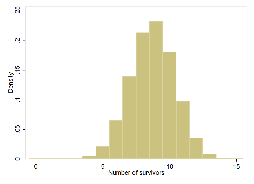
My results are:

4.091e-08  
2.647e-06  
.00006039  
.00069791  
.00479963  
.02141555  
.06519699  
.13945642  
.21276277  
.23238555  
.18045155  
.09775029  
.03565983  
.00823336  
.0010688  
.00005826  

Prob for # of survivors

The sum of the first three is the prob of being critically endangered, the last 5, the prob of least concern, etc.

$\endgroup$
2
  • $\begingroup$ Thank you, @StasK, this also looks like a good solution. +1 for the algorithm. $\endgroup$ Commented Oct 26, 2012 at 18:22
  • 2
    $\begingroup$ (+1) This is identical to the convolution solution I posted, except the convolutions are performed directly rather than with a built-in convolution function. There's little reason to prefer one method over the other for 15 probabilities, but with, say, 150000 of them, you might want to look at using an FFT. I had the same suspicions as you about numerical error creeping in, which is why I did the Mathematica comparison: it used exact arithmetic and its answers--fractions with large numerators and denominators--were converted to machine precision only at the end. The agreement was great. $\endgroup$
    – whuber
    Commented Oct 26, 2012 at 18:59
21
$\begingroup$

It's unclear what "risk of extinction category" means, but it appears the question asks to compute the distribution of the sum of 15 independent binomial variates having the given expectations. This is a convolution and it's most efficiently done with the Fast Fourier Transform.

Here is an example in R, whose convolve function uses the FFT:

x <- c(0.17,0.46,0.62,0.08,0.40,0.76,0.03,0.47,0.53,0.32,0.21,0.85,0.31,0.38,0.69)
z <- 1
for (u in sort(x)) z <- convolve(z, c(u, 1-u), type="open")
z

[1] 5.826e-05 1.069e-03 8.233e-03 3.566e-02 9.775e-02 1.805e-01 2.324e-01 2.128e-01

[9] 1.395e-01 6.520e-02 2.142e-02 4.800e-03 6.979e-04 6.039e-05 2.647e-06 4.091e-08

As a check, in Mathematica the same results were obtained with

Product[1 - z + z t, {z, x}] // Expand

$4.091095\times 10^{-8} t^{15}+2.647052\times 10^{-6} t^{14}+\cdots+0.0010688 t+0.0000582614$

Now, for instance, the chance of $10$ or fewer poisonings is computed in R as

sum(z[1:11])

[1] 0.9944

Edit

Using R's convolve function is inefficient for larger problems, because it repeatedly performs an FFT and its inverse. It turns out that the direct algorithm for convolution--as described by StasK--is plenty fast enough. Here is an R implementation.

convolve.binomial <- function(p) {
  # p is a vector of probabilities of Bernoulli distributions.
  # The convolution of these distributions is returned as a vector
  # `z` where z[i] is the probability of i-1, i=1, 2, ..., length(p)+1.
  n <- length(p) + 1
  z <- c(1, rep(0, n-1))
  for (p in p) z <- (1-p)*z + p*c(0, z[-n])
  return(z)
}

(Thanks to an anonymous editor suggesting improvements that clarify the algorithm.)

This takes $O(n^2)$ time for $n$ distributions--the quadratic behavior is not good--but it's still quite fast. As an example, let's generate 10,000 random probabilities (instead of using 15 given ones) and form the convolution of the corresponding Bernoulli distributions:

x <- runif(10000)
system.time(y <- convolve.binomial(x))

This still takes less than 3 seconds.

$\endgroup$
12
  • $\begingroup$ Thanks for your elegant solution, @whuber! You were correct in your understanding of "risk of extinction category"; since it could potentially be confusing and doesn't add anything to the question, I have removed those references. $\endgroup$ Commented Oct 26, 2012 at 18:13
  • 2
    $\begingroup$ I would accept both answers if I could as both answer the question comprehensively! Your answer was more immediately useful, while @StasK's solution was more instructive. On that basis I will select his answer as the most relevant to the question. But I appreciate the time and insight that you have both contributed. $\endgroup$ Commented Oct 27, 2012 at 22:28
  • 1
    $\begingroup$ Thanks from an old guy who never took college level probability courses. I've tried learning this stuff from textbooks, but having the capacity to play around with it in R makes it more immediate. I will try to link up this experience with my copies of Feller's wonderful volumes. $\endgroup$
    – DWin
    Commented Dec 2, 2013 at 19:43
  • 1
    $\begingroup$ @Antoni, each step adds a Bernoulli$(q)$ variable to the discrete variable whose probability generating function (pgf) is given in the variable z. If you like, think of z as representing the polynomial $z(t)=z_1+z_2t+z_3t^2+\cdots+z_nt^{n-1}$. The pgf of the Bernoulli variable is $f_q(t)=(1-q)+qt$. Each step of sapply computes an update $z(t)\to z(t)f_q(t)$. The initial value is $z(t)=1$. Thus, given the vector $\mathbf{p}=(p[1],p[2],\ldots,p[n-1])$, the loop computes the product $$\prod_{i=1}^{n-1}f_{p[i]}(t),$$ which is a polynomial of degree $n-1$ (therefore with $n$ coefficients). $\endgroup$
    – whuber
    Commented Oct 1, 2016 at 20:40
  • 1
    $\begingroup$ I did something almost identical to your convolve.binomial function. Just to note that it gives the probabilities for the numbers poisoned while StasK's chart is for the numbers surviving. $\endgroup$
    – Henry
    Commented Dec 13, 2022 at 17:06

Your Answer

By clicking “Post Your Answer”, you agree to our terms of service and acknowledge you have read our privacy policy.

Not the answer you're looking for? Browse other questions tagged or ask your own question.