5
$\begingroup$

Perhaps a very basic question but one that has me confused. Say, in a correlation table the relationship between A and the DV (B) is .351, but -.150 in the OLS model (where you have added C, D and E variables), what does this then mean? In other words: if the C to E variables not only change the coefficient of A but even make it go from negative to positive, does that indicate an undesirable interaction effect between the variables used in the OLS? I have been checking the VIF scores for this but based on low VIF I have no reason to fear multicollinearity. What (if anything) is wrong?

I'm trying to wrap my head around this constructing a simple example for myself to understand. Say A is a person's height and B is the distance this person jumps. There probably is a positive correlation (higher means longer legs, means longer distance jumping). What variables C to E would offset this person's height, even to the extent that this person's height is working against him when jumping (making the coefficient between A and DV B in the OLS negative)?

$\endgroup$
1
  • $\begingroup$ Why does a sign change disturbs you more than a mere change of magnitude? $\endgroup$
    – Gala
    Commented Jun 18, 2013 at 21:31

2 Answers 2

7
$\begingroup$

No, this doesn't imply 'the model is wrong' in the least. It's telling you that you should be wary of interpreting raw correlations when other important variables exist.

Here's a set of data I just generated (in R). The sample correlation between y and x1 is negative:

 print(cor(cbind(y,x1,x2)),d=3)
         y      x1     x2
y   1.0000 -0.0772 -0.830
x1 -0.0772  1.0000  0.196
x2 -0.8299  0.1961  1.000

Yet the coefficient in the regression is positive:

 summary(lm(y~x1+x2))

... [snip]

Coefficients:
            Estimate Std. Error t value Pr(>|t|)    
(Intercept)  11.8231     2.6183   4.516 9.73e-05 ***
x1            0.1203     0.1412   0.852    0.401    
x2           -5.8462     0.7201  -8.119 5.94e-09 ***
---
Signif. codes:  0 ‘***’ 0.001 ‘**’ 0.01 ‘*’ 0.05 ‘.’ 0.1 ‘ ’ 1

Residual standard error: 4.466 on 29 degrees of freedom
Multiple R-squared:  0.6963,    Adjusted R-squared:  0.6753 
F-statistic: 33.24 on 2 and 29 DF,  p-value: 3.132e-08

Is the 'model' wrong? No, I fitted the same model I used to create the data, one that satisfies all the regression assumptions,

$y = 9 + 0.2 x_1 - 5 x_2 + e $, where $e_i \sim N(0,4^2)$,

or in R: y= 9 + 0.2*x1 -5*x2 + rnorm(length(x2),0,4)

So how does this happen?

Look at two things. First, look at the plot of $y$ vs $x_1$:
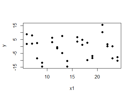
y vs x1

And we see a (very slight in this case) negative correlation.

Now look at the same plot, but with the values at a particular value of $x_2$ ($x_2=4$) marked in red:
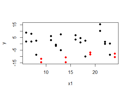
y vs x1, x2=4 marked in red

... at a given value of $x_2$, the relationship with $x_1$ is increasing, not decreasing. The same happens at the other values of $x_2$. For each value of $x_2$, the relationship between $y$ and $x_1$ is positive. So why is the correlation negative? Because $x_1$ and $x_2$ are related.

If we want to look at correlation and have it correspond to the regression, the partial correlation rather than the raw correlation is the relevant quantity; here's the table of partial correlations (using package ppcor):

 print(pcor(cbind(y,x1,x2))$estimate,d=3)
        y    x1     x2
y   1.000 0.156 -0.833
x1  0.156 1.000  0.237
x2 -0.833 0.237  1.000

We see the partial correlation between $y$ and $x_1$ controlling for $x_2$ is positive.

It wasn't the regression results that one had to beware of, it was the misleading impression from looking at the raw correlation.

Incidentally, it's also quite possible to make it so both the correlation and regression coefficient are significantly different from zero and of opposite sign ... and there's still nothing wrong with the model.

$\endgroup$
5
$\begingroup$

In addition to looking at the coefficients, you should also look at their confidence intervals. If the interval is quite wide then a change from $0.351$ to $-0.150$ could be explained by random chance. Even if the intervals are narrow (and show significant difference) a change in sign is not uncommon.

Remember that the interpretation of a single slope is the effect of changing that variable while holding all others constant. Even with moderate correlation (well below the level that would cause a VIF to be interesting) this can be an unreasonable assumption that does not help with interpretation and can lead to the reversal. Think of what it means to increase someone's height while keeping their weight constant.

Another example. $Y$ is the value of all the coins in a person's pocket, $X_1$ is the total number of coins, $X_2$ is the number of coins in the pocket that are not quarters (or the highest common denomination of coin for the region). We would expect positive correlation between all 3 variables, but if we hold $X_1$ constant and increase $X_2$ then $Y$ would decrease.

$\endgroup$

Your Answer

By clicking “Post Your Answer”, you agree to our terms of service and acknowledge you have read our privacy policy.

Not the answer you're looking for? Browse other questions tagged or ask your own question.