Wilcoxon Rank Sum (Mann Whitney) test-SAS Results Interpretation

Question

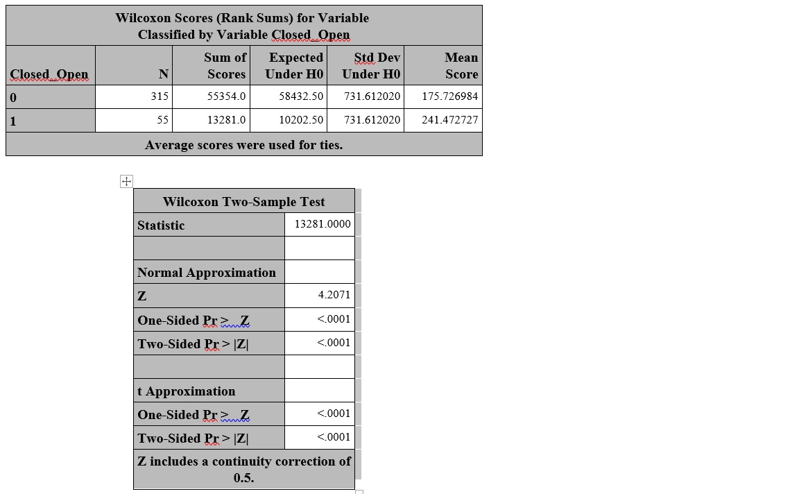
I need a clarification on interpreting Wilcoxon Rank Sum (Mann Whitney) test results using SAS. Here is a sample results look like. I am trying to form a hypothesis and interpret the results. In this case, is this the test for average or medians, since the results display the mean score. Also should I use the normal approximation or t approximation for the p-value.

Answer 1

There are two Wilcoxon tests, which can lead to some confusion. However, both are non-parametric tests that are not median value tests but are difference of locations tests. The Wilcoxon rank-sum test is often called the Mann-Whitney U test and is used to compare independent random variables. Click on that link to find out more about what that test does. Briefly, this tests the whether two groups of subjects with unequal numbers of subjects in each group, have the same location. It is not sensitive to non-normal conditions, thus its popularity.

Interpretation: As a test of location, one tests whether the data location is the same for two independent populations. The null hypothesis implies that there is a significant difference in location of the populations, and the alternative hypothesis implies that a significant difference was not detected under the conditions of the test. When the probability of this test is low [most often $p<0.05$, with a Type I error (AKA alpha, false positive rate) set at 0.05] we would accept the null (H0) hypothesis as the likelihood of the alternative hypothesis (H1) is low.

The second test is for paired data, and it compares "before" and "after" effects on the same subjects. This is called the Wilcoxon signed-rank test, which is not a synonym for the other Wilcoxon test, the Wilcoxon rank-sum test. The interpretation of this test is similar that of the other test above with the exception that there is no independence, the test is more sensitive for detecting differences, and the data has the same number of "participants" in both groups.

The Mann-Whitney U test uses the U-statistic as a measure of location. "U" stands for Unbiased. Such statistics arise in the context of minimum variance unbiased estimators, or UVME for short. The U-statistic has the property that the average over sample values $ƒ_n(x\phi)$ is exactly equal to the population value $ƒ_N(x)$ for a simple random sample $\phi$ of size $n$ taken from a population of size $N$.

Keep in mind that the Mann-Whitney U test is non-parametric, that is, it uses yes/no comparisons between entries and not distances. The U statistic, for that test, corresponds to the number of wins (> versus <) out of all pairwise contests. For each observation in one set, count the number of times this first value wins over any observations in the other set (the other value loses if this first is larger). Count 0.5 for any ties. The sum of wins and ties is U for the first set. U for the other set is the converse. One then uses a lookup table to convert U into probabilities. For larger sample size, say >20, there is a normal approximation for p(U).

This test works because the group of binary comparisons used results in a symmetric distribution for which the probabilities of difference of locations are calculable, even though the original data may consist of two asymmetrically distributed populations for which probabilities of difference of location are not easily calculable. Since the entries must be amenable to comparison of the >, < or = type, at least ordinal data is required, where by ordinal we mean non-parametric data for which > and < is a property, e.g., "How do you like my answer?" 1) Very dissatisfied 2) Somewhat dissatisfied 3) So-so 4) Somewhat satisfied 5) Very satisfied.