What intuitive explanation is there for the central limit theorem?

Question

In several different contexts we invoke the central limit theorem to justify whatever statistical method we want to adopt (e.g., approximate the binomial distribution by a normal distribution). I understand the technical details as to why the theorem is true but it just now occurred to me that I do not really understand the intuition behind the central limit theorem.

So, what is the intuition behind the central limit theorem?

Layman explanations would be ideal. If some technical detail is needed please assume that I understand the concepts of a pdf, cdf, random variable etc but have no knowledge of convergence concepts, characteristic functions or anything to do with measure theory.

Answer 1

I apologize in advance for the length of this post: it is with some trepidation that I let it out in public at all, because it takes some time and attention to read through and undoubtedly has typographic errors and expository lapses. But here it is for those who are interested in the fascinating topic, offered in the hope that it will encourage you to identify one or more of the many parts of the CLT for further elaboration in responses of your own.

---

Most attempts at "explaining" the CLT are illustrations or just restatements that assert it is true. A really penetrating, correct explanation would have to explain an awful lot of things.

Before looking at this further, let's be clear about what the CLT says. As you all know, there are versions that vary in their generality. The common context is a sequence of random variables, which are certain kinds of functions on a common probability space. For intuitive explanations that hold up rigorously I find it helpful to think of a probability space as a box with distinguishable objects. It doesn't matter what those objects are but I will call them "tickets." We make one "observation" of a box by thoroughly mixing up the tickets and drawing one out; that ticket constitutes the observation. After recording it for later analysis we return the ticket to the box so that its contents remain unchanged. A "random variable" basically is a number written on each ticket.

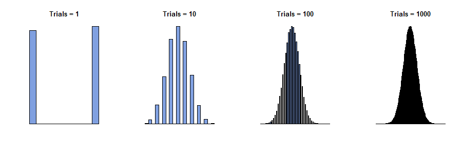
In 1733, Abraham de Moivre considered the case of a single box where the numbers on the tickets are only zeros and ones ("Bernoulli trials"), with some of each number present. He imagined making $n$ physically independent observations, yielding a sequence of values $x_1, x_2, \ldots, x_n$, all of which are zero or one. The sum of those values, $y_n = x_1 + x_2 + \ldots + x_n$, is random because the terms in the sum are. Therefore, if we could repeat this procedure many times, various sums (whole numbers ranging from $0$ through $n$) would appear with various frequencies--proportions of the total. (See the histograms below.)

Now one would expect--and it's true--that for very large values of $n$, all the frequencies would be quite small. If we were to be so bold (or foolish) as to attempt to "take a limit" or "let $n$ go to $\infty$", we would conclude correctly that all frequencies reduce to $0$. But if we simply draw a histogram of the frequencies, without paying any attention to how its axes are labeled, we see that the histograms for large $n$ all begin to look the same: in some sense, these histograms approach a limit even though the frequencies themselves all go to zero.

These histograms depict the results of repeating the procedure of obtaining $y_n$ many times. $n$ is the "number of trials" in the titles.

The insight here is to draw the histogram first and label its axes later. With large $n$ the histogram covers a large range of values centered around $n/2$ (on the horizontal axis) and a vanishingly small interval of values (on the vertical axis), because the individual frequencies grow quite small. Fitting this curve into the plotting region has therefore required both a shifting and rescaling of the histogram. The mathematical description of this is that for each $n$ we can choose some central value $m_n$ (not necessarily unique!) to position the histogram and some scale value $s_n$ (not necessarily unique!) to make it fit within the axes. This can be done mathematically by changing $y_n$ to $z_n = (y_n - m_n) / s_n$.

Remember that a histogram represents frequencies by areas between it and the horizontal axis. The eventual stability of these histograms for large values of $n$ should therefore be stated in terms of area. So, pick any interval of values you like, say from $a$ to $b \gt a$ and, as $n$ increases, track the area of the part of the histogram of $z_n$ that horizontally spans the interval $(a, b]$. The CLT asserts several things:

1. No matter what $a$ and $b$ are, if we choose the sequences $m_n$ and $s_n$ appropriately (in a way that does not depend on $a$ or $b$ at all), this area indeed approaches a limit as $n$ gets large.

2. The sequences $m_n$ and $s_n$ can be chosen in a way that depends only on $n$, the average of values in the box, and some measure of spread of those values--but on nothing else--so that regardless of what is in the box, the limit is always the same. (This universality property is amazing.)

3. Specifically, that limiting area is the area under the curve $y = \exp(-z^2/2) / \sqrt{2 \pi}$ between $a$ and $b$: this is the formula of that universal limiting histogram.

The first generalization of the CLT adds,

4. When the box can contain numbers in addition to zeros and ones, exactly the same conclusions hold (provided that the proportions of extremely large or small numbers in the box are not "too great," a criterion that has a precise and simple quantitative statement).

The next generalization, and perhaps the most amazing one, replaces this single box of tickets with an ordered indefinitely long array of boxes with tickets. Each box can have different numbers on its tickets in different proportions. The observation $x_1$ is made by drawing a ticket from the first box, $x_2$ comes from the second box, and so on.

5. Exactly the same conclusions hold provided the contents of the boxes are "not too different" (there are several precise, but different, quantitative characterizations of what "not too different" has to mean; they allow an astonishing amount of latitude).

These five assertions, at a minimum, need explaining. There's more. Several intriguing aspects of the setup are implicit in all the statements. For example,

• What is special about the sum? Why don't we have central limit theorems for other mathematical combinations of numbers such as their product or their maximum? (It turns out we do, but they are not quite so general nor do they always have such a clean, simple conclusion unless they can be reduced to the CLT.) The sequences of $m_n$ and $s_n$ are not unique but they're almost unique in the sense that eventually they have to approximate the expectation of the sum of $n$ tickets and the standard deviation of the sum, respectively (which, in the first two statements of the CLT, equals $\sqrt{n}$ times the standard deviation of the box).

  The standard deviation is one measure of the spread of values, but it is by no means the only one nor is it the most "natural," either historically or for many applications. (Many people would choose something like a median absolute deviation from the median, for instance.)

• Why does the SD appear in such an essential way?

• Consider the formula for the limiting histogram: who would have expected it to take such a form? It says the logarithm of the probability density is a quadratic function. Why? Is there some intuitive or clear, compelling explanation for this?

---

I confess I am unable to reach the ultimate goal of supplying answers that are simple enough to meet Srikant's challenging criteria for intuitiveness and simplicity, but I have sketched this background in the hope that others might be inspired to fill in some of the many gaps. I think a good demonstration will ultimately have to rely on an elementary analysis of how values between $\alpha_n = a s_n + m_n$ and $\beta_n = b s_n + m_n$ can arise in forming the sum $x_1 + x_2 + \ldots + x_n$. Going back to the single-box version of the CLT, the case of a symmetric distribution is simpler to handle: its median equals its mean, so there's a 50% chance that $x_i$ will be less than the box's mean and a 50% chance that $x_i$ will be greater than its mean. Moreover, when $n$ is sufficiently large, the positive deviations from the mean ought to compensate for the negative deviations in the mean. (This requires some careful justification, not just hand waving.) Thus we ought primarily to be concerned about counting the numbers of positive and negative deviations and only have a secondary concern about their sizes. (Of all the things I have written here, this might be the most useful at providing some intuition about why the CLT works. Indeed, the technical assumptions needed to make the generalizations of the CLT true essentially are various ways of ruling out the possibility that rare huge deviations will upset the balance enough to prevent the limiting histogram from arising.)

This shows, to some degree anyway, why the first generalization of the CLT does not really uncover anything that was not in de Moivre's original Bernoulli trial version.

At this point it looks like there is nothing for it but to do a little math: we need to count the number of distinct ways in which the number of positive deviations from the mean can differ from the number of negative deviations by any predetermined value $k$, where evidently $k$ is one of $-n, -n+2, \ldots, n-2, n$. But because vanishingly small errors will disappear in the limit, we don't have to count precisely; we only need to approximate the counts. To this end it suffices to know that

$$\text{The number of ways to obtain } k \text{ positive and } n-k \text{ negative values out of } n$$

$$\text{equals } \frac{n-k+1}{k}$$

$$\text{times the number of ways to get } k-1 \text{ positive and } n-k+1 \text { negative values.}$$

(That's a perfectly elementary result so I won't bother to write down the justification.) Now we approximate wholesale. The maximum frequency occurs when $k$ is as close to $n/2$ as possible (also elementary). Let's write $m = n/2$. Then, relative to the maximum frequency, the frequency of $m+j+1$ positive deviations ($j \ge 0$) is estimated by the product

$$\frac{m+1}{m+1} \frac{m}{m+2} \cdots \frac{m-j+1}{m+j+1}$$

$$=\frac{1 - 1/(m+1)}{1 + 1/(m+1)} \frac{1-2/(m+1)}{1+2/(m+1)} \cdots \frac{1-j/(m+1)}{1+j/(m+1)}.$$

135 years before de Moivre was writing, John Napier invented logarithms to simplify multiplication, so let's take advantage of this. Using the approximation

$$\log\left(\frac{1-x}{1+x}\right) = -2x - \frac{2x^3}{3} + O(x^5),$$

we find that the log of the relative frequency is approximately

$$-\frac{2}{m+1}\left(1 + 2 + \cdots + j\right) - \frac{2}{3(m+1)^3}\left(1^3+2^3+\cdots+j^3\right) = -\frac{j^2}{m} + O\left(\frac{j^4}{m^3}\right).$$

Because the error in approximating this sum by $-j^2/m$ is on the order of $j^4/m^3$, the approximation ought to work well provided $j^4$ is small relative to $m^3$. That covers a greater range of values of $j$ than is needed. (It suffices for the approximation to work for $j$ only on the order of $\sqrt{m}$ which asymptotically is much smaller than $m^{3/4}$.)

Consequently, writing $$z = \sqrt{2}\,\frac{j}{\sqrt{m}} = \frac{j/n}{1 / \sqrt{4n}}$$ for the standardized deviation, the relative frequency of deviations of size given by $z$ must be proportional to $\exp(-z^2/2)$ for large $m.$ Thus appears the Gaussian law of #3 above.

---

Obviously much more analysis of this sort should be presented to justify the other assertions in the CLT, but I'm running out of time, space, and energy and I've probably lost 90% of the people who started reading this anyway. This simple approximation, though, suggests how de Moivre might originally have suspected that there is a universal limiting distribution, that its logarithm is a quadratic function, and that the proper scale factor $s_n$ must be proportional to $\sqrt{n}$ (as shown by the denominator of the preceding formula). It is difficult to imagine how this important quantitative relationship could be explained without invoking some kind of mathematical information and reasoning; anything less would leave the precise shape of the limiting curve a complete mystery.

Answer 2

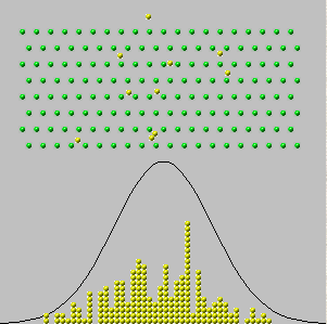
The nicest animation I know: http://www.ms.uky.edu/~mai/java/stat/GaltonMachine.html

The simplest words I have read: http://elonen.iki.fi/articles/centrallimit/index.en.html

If you sum the results of these ten throws, what you get is likely to be closer to 30-40 than the maximum, 60 (all sixes) or on the other hand, the minumum, 10 (all ones).

The reason for this is that you can get the middle values in many more different ways than the extremes. Example: when throwing two dice: 1+6 = 2+5 = 3+4 = 7, but only 1+1 = 2 and only 6+6 = 12.

That is: even though you get any of the six numbers equally likely when throwing one die, the extremes are less probable than middle values in sums of several dice.

Answer 3

An observation concerning the CLT may be the following. When you have a sum $$ S = X_1 + X_2 + \ldots + X_n $$ of a lot of random components, if one is "smaller than usual" then this is mostly compensated for by some of the other components being "larger than usual". In other words, negative deviations and positive deviations from the component means cancel each other out in the summation. Personally, I have no clear-cut intuition why exactly the remaining deviations form a distribution that looks more and more normal the more terms you have.

There are many versions of the CLT, some stronger than others, some with relaxed conditions such as a moderate dependence between the terms and/or non-identical distributions for the terms. In the simplest-to-prove versions of the CLT, the proof is usually based on the moment-generating function (or Laplace-Stieltjes transform or some other appropriate transform of the density) of the sum $S$. Writing this as a Taylor expansion and keeping only the most dominant term gives you the moment-generating function of the normal distribution. So for me personally, the normality is something that follows from a bunch of equations and I can not provide any further intuition than that.

It should be noted however that the sum's distribution, never really is normally distributed, nor does the CLT claims that it would be. If $n$ is finite, there is still some distance to the normal distribution and if $n=\infty$ both the mean and the variance are infinite as well. In the latter case you could take the mean of the infinite sum, but then you get a deterministic number without any variance at all, which could hardly be labelled as "normally distributed".

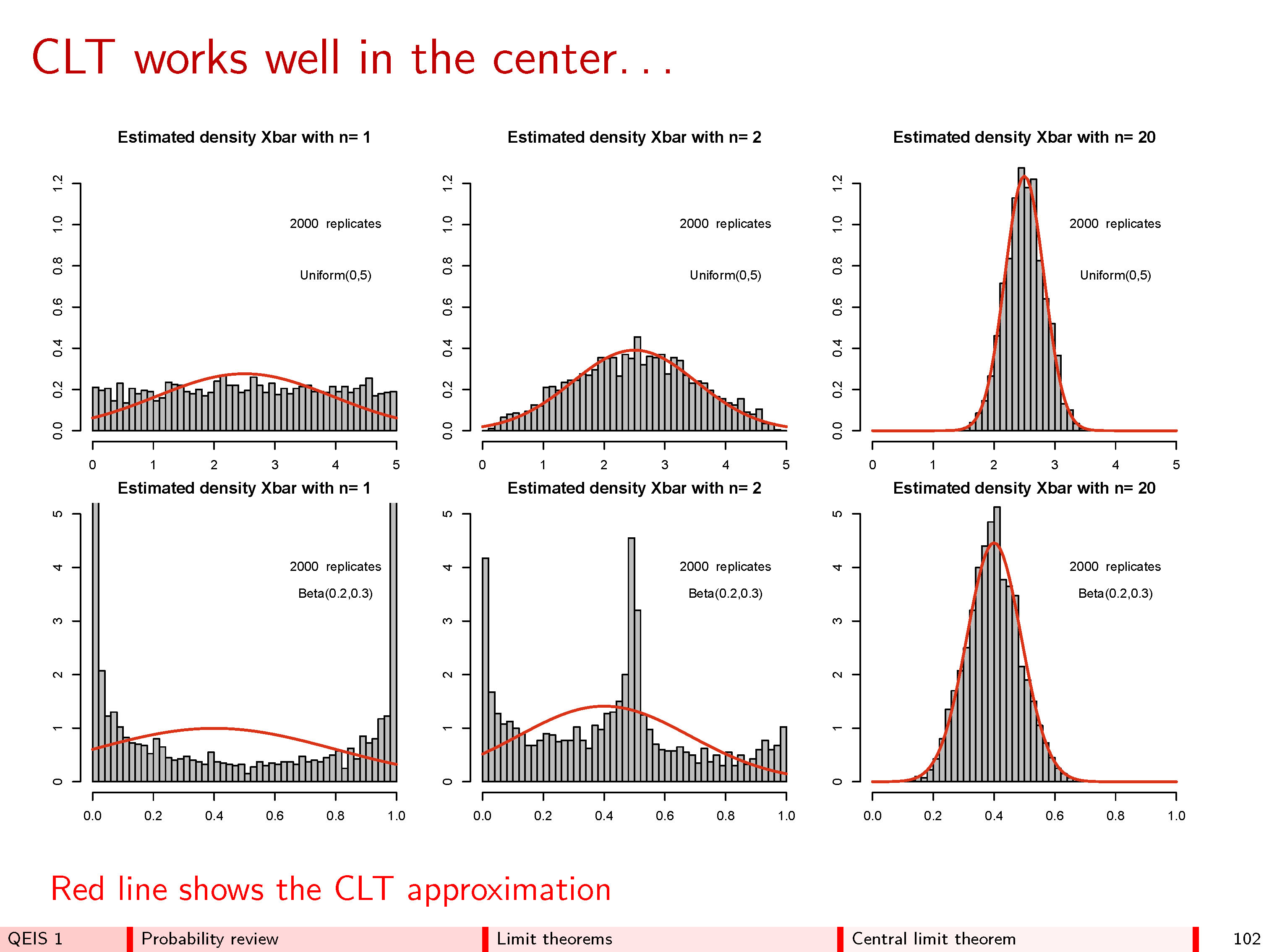
This may pose problems with practical applications of the CLT. Usually, if you are interested in the distribution of $S/n$ close to its center, CLT works fine. However, convergence to the normal is not uniform everywhere and the further you get away from the center, the more terms you need to have a reasonable approximation.

With all the "sanctity" of the Central Limit Theorem in statistics, its limitations are often overlooked all too easily. Below I give two slides from my course making the point that CLT utterly fails in the tails, in any practical use case. Unfortunately, a lot of people specifically use CLT to estimate tail probabilities, knowingly or otherwise.

Answer 4

Intuition is a tricky thing. It's even trickier with theory in our hands tied behind our back.

The CLT is all about sums of tiny, independent disturbances. "Sums" in the sense of the sample mean, "tiny" in the sense of finite variance (of the population), and "disturbances" in the sense of plus/minus around a central (population) value.

For me, the device that appeals most directly to intuition is the quincunx, or 'Galton box', see Wikipedia (for 'bean machine'?) The idea is to roll a tiny little ball down the face of a board adorned by a lattice of equally spaced pins. On its way down the ball diverts right and left (...randomly, independently) and collects at the bottom. Over time, we see a nice bell shaped mound form right before our eyes.

The CLT says the same thing. It is a mathematical description of this phenomenon (more precisely, the quincunx is physical evidence for the normal approximation to the binomial distribution). Loosely speaking, the CLT says that as long as our population is not overly misbehaved (that is, if the tails of the PDF are sufficiently thin), then the sample mean (properly scaled) behaves just like that little ball bouncing down the face of the quincunx: sometimes it falls off to the left, sometimes it falls off to the right, but most of the time it lands right around the middle, in a nice bell shape.

The majesty of the CLT (to me) is that the shape of the underlying population is irrelevant. Shape only plays a role insofar as it delegates the length of time we need to wait (in the sense of sample size).

Answer 5

This answer hopes to give an intuitive meaning of the central limit theorem, using simple calculus techniques (Taylor expansion of order 3). Here is the outline:

1. What the CLT says
2. An intuitive proof of the CLT using simple calculus
3. Why the normal distribution?

We will mention the normal distribution at the very end; because the fact that the normal distribution eventually comes up does not bear much intuition.

1. What the central limit theorem says? Several versions of the CLT

There are several equivalent versions of the CLT. The textbook statement of the CLT says that for any real $x$ and any sequence of independent random variables $X_1,\cdots,X_n$ with zero-mean and variance 1, \[P\left(\frac{X_1+\cdots+X_n}{\sqrt n} \le x\right) \to_{n\to+\infty} \int_{-\infty}^x \frac{e^{-t^2/2}}{\sqrt{2\pi}} dt.\] To understand on what is universal and intuitive about the CLT, let's forget the limit for a moment. The above statement says that if $X_1.,\ldots,X_n$ and $Z_1,\ldots,Z_n$ are two sequences of independent random variables each with zero-mean and variance 1, then \[E \left[ f\left(\tfrac{X_1+\cdots+X_n}{\sqrt n}\right) \right] - E \left[ f\left(\tfrac{Z_1+\cdots+Z_n}{\sqrt n}\right) \right] \to_{n\to+\infty} 0 \] for every indicator function $f$ of the form, for some fixed real $x$, \begin{equation} f(t) = \begin{cases} 1 \text{ if } t < x \\ 0 \text{ if } t\ge x.\end{cases} \end{equation} The previous display embodies the fact the limit is the same no matter the particular distributions of $X_1,\ldots,X_n$ and $Z_1,\ldots,Z_n$, provided that the random variables are independent with mean zero, variance one.

Some other versions of the CLT mentions the class of Lipschtiz functions that are bounded by 1; some other versions of the CLT mentions the class of smooth functions with bounded derivative of order $k$. Consider two sequences $X_1,\ldots,X_n$ and $Z_1,\ldots,Z_n$ as above, and for some function $f$, the convergence result (CONV)

\[E \left[ f\left(\tfrac{X_1+\cdots+X_n}{\sqrt n}\right) \right] - E \left[ f\left(\tfrac{Z_1+\cdots+Z_n}{\sqrt n}\right) \right] \to_{n\to+\infty} 0 \tag{CONV}\]

It is possible to establish the equivalence ("if and only if") between the following statements:

1. (CONV) above holds for every indicator functions $f$ of the form $f(t)=1$ for $t < x$ and $f(t)=0$ for $t\ge x$ for some fixed real $x$.
2. (CONV) holds for every bounded lipschitz function $f:R\to R$.
3. (CONV) holds for every smooth (i.e., $C^{\infty}$) functions with compact support.
4. (CONV) holds for every functions $f$ three time continuously differentiable with $\sup_{x\in R} |f'''(x)| \le 1$.

Each of the 4 points above says that the convergence holds for a large class of functions. By a technical approximation argument, one can show that the four points above are equivalent, we refer the reader to Chapter 7, page 77 of David Pollard's book A user's guide to measure theoretic probabilities from which this answer is highly inspired.

Our assumption for the remaining of this answer...

We will assume that $\sup_{x\in R} |f'''(x)| \le C$ for some constant $C>0$, which corresponds to point 4 above. We will also assume that the random variables have finite, bounded third moment: $E[|X_i|^3]$ and $E[|Z_i|^3]$ are finite.

2. The value of $E\left[ f\left( \tfrac{X_1+\cdots+X_n}{\sqrt n} \right) \right]$ is universal: it does not depend on the distribution of $X_1,...,X_n$

Let us show that this quantity is universal (up to a small error term), in the sense that it does not depend on which collection of independent random variables was provided. Take $X_1,\ldots,X_n$ and $Z_1,\ldots,Z_n$ two sequences of independent random variables, each with mean 0 and variance 1, and finite third moment.

The idea is to iteratively replace $X_i$ by $Z_i$ in one of the quantity and control the difference by basic calculus (the idea, I believe, is due to Lindeberg). By a Taylor expansion, if $W = Z_1+\cdots+Z_{n-1}$, and $h(x)=f(x/\sqrt n)$ then \begin{align} h(Z_1+\cdots+Z_{n-1}+X_n) &= h(W) + X_n h'(W) + \frac{X_n^2 h''(W)}{2} + \frac{X_n^3/h'''(M_n)}{6} \\ h(Z_1+\cdots+Z_{n-1}+Z_n) &= h(W) + Z_n h'(W) + \frac{Z_n^2 h''(W)}{2} + \frac{Z_n^3 h'''(M_n')}{6} \\ \end{align} where $M_n$ and $M_n'$ are midpoints given by the mean-value theorem. Taking expectation on both lines, the zeroth order term is the same, the first order terms are equal in expectation because by independence of $X_n$ and $W$, $E[X_n h'(W)]= E[X_n] E[h'(W)] =0$ and similarly for the second line. Again by independence, the second order terms are the same in expectation. The only remaining terms are the third order one, and in expectation the difference between the two lines is at most \[ \frac{(C/6)E[ |X_n|^3 + |Z_n|^3 ]}{(\sqrt n)^3}. \] Here $C$ is an upper bound on the third derivative of $f'''$. The denominator $(\sqrt{n})^3$ appears because $h'''(t) = f'''(t/\sqrt n)/(\sqrt n)^3$. By independence, the contribution of $X_n$ in the sum is meaningless because it could be replaced by $Z_n$ without incurring an error larger than the above display!

We now reiterate to replace $X_{n-1}$ by $Z_{n-1}$. If $\tilde W= Z_1+Z_2+\cdots+Z_{n-2} + X_n$ then \begin{align} h(Z_1+\cdots+Z_{n-2}+X_{n-1}+X_n) &= h(\tilde W) + X_{n-1} h'(\tilde W) + \frac{X_{n-1}^2 h''(\tilde W)}{2} + \frac{X_{n-1}^3/h'''(\tilde M_n)}{6}\\ h(Z_1+\cdots+Z_{n-2}+Z_{n-1}+X_n) &= h(\tilde W) + Z_{n-1} h'(\tilde W) + \frac{Z_{n-1}^2 h''(\tilde W)}{2} + \frac{Z_{n-1}^3/h'''(\tilde M_n)}{6}. \end{align} By independence of $Z_{n-1}$ and $\tilde W$, and by independence of $X_{n-1}$ and $\tilde W$, again the zeroth, first and second order terms are equal in expectation for both lines. The difference in expectation between the two lines is again at most \[ \frac{(C/6)E[ |X_{n-1}|^3 + |Z_{n-1}|^3 ]}{(\sqrt n)^3}. \] We keep iterating until we replaced all $Z_i$'s with $X_i$'s. By adding the errors made at each of the $n$ steps, we obtain \[ \Big| E\left[ f\left( \tfrac{X_1+\cdots+X_n}{\sqrt n} \right) \right]-E\left[ f\left( \tfrac{Z_1+\cdots+Z_n}{\sqrt n} \right) \right] \Big| \le n \frac{(C/6)\max_{i=1,\ldots,n} E[ |X_i|^3 + |Z_i|^3 ]}{(\sqrt n)^3}. \] as $n$ increases, the right hand side converges to 0 if the third moments of our random variables are finite (let's assume it is the case). This means that the expectations on the left become arbitrarily close to each other, no matter if the distribution of $X_1,\ldots,X_n$ is far from that of $Z_1,\ldots,Z_n$. By independence, the contribution of each $X_i$ in the sum is meaningless because it could be replaced by $Z_i$ without incurring an error larger than $O(1/(\sqrt n)^3)$. And replacing all $X_i$'s by the $Z_i$'s does not change the quantity by more than $O(1/\sqrt n)$.

The expectation $E\left[ f\left( \frac{X_1+\cdots+X_n}{\sqrt n} \right) \right]$ is thus universal, it does not depend on the distribution of $X_1,\ldots,X_n$. On the other hand, independence and $E[X_i]=E[Z_i]=0,E[Z_i^2]=E[X_i^2]=1$ was of utmost importance for the above bounds.

3. Why the normal distribution?

We have seen that the expectation $E\left[ f\left( \frac{X_1+\cdots+X_n}{\sqrt n} \right) \right]$ will be the same no matter what the distribution of $X_i$ is, up to a small error of order $O(1/\sqrt n)$.

But for applications, it would be useful to compute such quantity. It would also be useful to get a simpler expression for this quantity $E\left[ f\left( \frac{X_1+\cdots+X_n}{\sqrt n} \right) \right]$.

Since this quantity is the same for any collection $X_1,\ldots,X_n$, we can simply pick one specific collection such that the distribution $(X_1+\cdots+X_n)/\sqrt n$ is easy to compute or easy to remember.

For the normal distribution $N(0,1)$, it happens that this quantity becomes really simple. Indeed, if $Z_1,\ldots,Z_n$ are iid $N(0,1)$ then $\frac{Z_1+\cdots+Z_n}{\sqrt n}$ has also the $N(0,1)$ distribution and it does not depend on $n$! Hence if $Z\sim N(0,1)$, then \[ E\left[ f\left( \frac{Z_1+\cdots+Z_n}{\sqrt n} \right) \right] = E[ f(Z)], \] and by the above argument, for any collection of independent random variables $X_1,\ldots,X_n$ with $E[X_i]=0,E[X_i^2]=1$, then

\[ \left| E\left[ f\left( \frac{X_1+\cdots+X_n}{\sqrt n} \right) \right] -E[f(Z) \right| \le \frac{\sup_{x\in R} |f'''(x)| \max_{i=1,\ldots,n} E[|X_i|^3 + |Z|^3]}{6\sqrt n}. \]

Answer 6

Why the $\sqrt{n}$ instead of $n$? What's this weird version of an average?

If you have a bunch of perpendicular vectors $x_1, \dotsc, x_n$ of length $\ell$, then $ \frac{x_1 + \dotsb + x_n}{\sqrt{n}}$ is again of length $\ell.$ You have to normalize by $\sqrt{n}$ to keep the sum at the same scale.

There is a deep connection between independent random variables and orthogonal vectors. When random variables are independent, that basically means that they are orthogonal vectors in a vector space of functions.

(The function space I refer to is $L^2$, and the variance of a random variable $X$ is just $\|X - \mu\|_{L^2}^2$. So no wonder the variance is additive over independent random variables. Just like $\|x + y\|^2 = \|x\|^2 + \|y\|^2$ when $x \perp y$.)**

Why the normal distribution?

One thing that really confused me for a while, and which I think lies at the heart of the matter, is the following question:

Why is it that the sum $\frac{X_1 + \dotsb + X_n} {\sqrt{n}}$ ($n$ large) doesn’t care anything about the $X_i$ except their mean and their variance? (Moments 1 and 2.)

This is similar to the law of large numbers phenomenon:

$\frac{X_1 + \dotsb + X_n} {n}$ ($n$ large) only cares about moment 1 (the mean).

(Both of these have their hypotheses that I'm suppressing (see the footnote), but the most important thing, of course, is that the $X_i$ be independent.)

A more elucidating way to express this phenomenon is: in the sum $\frac{X_1 + \dotsb + X_n}{\sqrt{n}}$, I can replace any or all of the $X_i$ with some other RV’s, mixing and matching between all kinds of various distributions, as long as they have the same first and second moments. And it won’t matter as long as $n$ is large, relative to the moments.

If we understand why that’s true, then we understand the central limit theorem. Because then we may as well take $X_i$ to be normal with the same first and second moment, and in that case we know $\frac{X_1 + \dotsb + X_n}{\sqrt{n}}$ is just normal again for any $n$, including super-large $n$. Because the normal distribution has the special property ("stability") that you can add two independent normals together and get another normal. Voila.

The explanation of the first-and-second-moment phenomemonon is ultimately just some arithmetic. There are several lenses through which once can choose to view this arithmetic. The most common one people use is the fourier transform (AKA characteristic function), which has the feel of "I follow the steps, but how and why would anyone ever think of that?" Another approach is to look at the cumulants of $X_i$. There we find that the normal distribution is the unique distribution whose higher cumulants vanish, and dividing by $\sqrt{n}$ tends to kill all but the first two cumulants as $n$ gets large.

I'll show here a more elementary approach. As the sum $Z_n \overset{\text{(def)}}{=} \frac{X_1 + \dotsb + X_n}{\sqrt{n}}$ gets longer and longer, I'll show that all of the moments of $Z_n$ are functions only of the variances $\operatorname{Var}(X_i)$ and the means $\mathbb{E}X_i$, and nothing else. Now the moments of $Z_n$ determine the distribution of $Z_n$ (that's true not just for long independent sums, but for any nice distribution, by the Carleman continuity theorem). To restate, we're claiming that as $n$ gets large, $Z_n$ depends only on the $\mathbb{E}X_i$ and the $\operatorname{Var}X_i$. And to show that, we're going to show that $\mathbb{E}((Z_n - \mathbb{E}Z_n)^k)$ depends only on the $\mathbb{E}X_i$ and the $\operatorname{Var}X_i$. That suffices, by the Carleman continuity theorem.

For convenience, let's require that the $X_i$ have mean zero and variance $\sigma^2$. Assume all their moments exist and are uniformly bounded. (But nevertheless, the $X_i$ can be all different independent distributions.)

Claim: Under the stated assumptions, the $k$th moment $$\mathbb{E} \left[ \left(\frac{X_1 + \dotsb + X_n}{\sqrt{n}}\right)^k \right]$$ has a limit as $n \to \infty$, and that limit is a function only of $\sigma^2$. (It disregards all other information.)

(Specifically, the values of those limits of moments are just the moments of the normal distribution $\mathcal{N}(0, \sigma^2)$: zero for $k$ odd, and $|\sigma|^k \frac{k!}{(k/2)!2^{k/2}}$ when $k$ is even. This is equation (1) below.)

Proof: Consider $\mathbb{E} \left[ \left(\frac{X_1 + \dotsb + X_n}{\sqrt{n}}\right)^k \right]$. When you expand it, you get a factor of $n^{-k/2}$ times a big fat multinomial sum.

$$n^{-k/2} \sum_{|\boldsymbol{\alpha}| = k} \binom{k}{\alpha_1, \dotsc, \alpha_n}\prod_{i=1}^n \mathbb{E}(X_i^{\alpha_i})$$ $$\alpha_1 + \dotsb + \alpha_n = k$$ $$(\alpha_i \geq 0)$$

(Remember you can distribute the expectation over independent random variables. $\mathbb{E}(X^a Y^b) = \mathbb{E}(X^a)\mathbb{E}(Y^b)$.)

Now if ever I have as one of my factors a plain old $\mathbb{E}(X_i)$, with exponent $\alpha_i =1$, then that whole term is zero, because $\mathbb{E}(X_i) = 0$ by assumption. So I need all the exponents $\alpha_i \neq 1$ in order for that term to survive. That pushes me toward using fewer of the $X_i$ in each term, because each term has $\sum \alpha_i = k$, and I have to have each $\alpha_i >1$ if it is $>0$. In fact, some simple arithmetic shows that at most $k/2$ of the $\alpha_i$ can be nonzero, and that's only when $k$ is even, and when I use only twos and zeros as my $\alpha_i$.

This pattern where I use only twos and zeros turns out to be very important...in fact, any term where I don't do that will vanish as the sum grows larger.

Lemma: The sum $$n^{-k/2} \sum_{|\boldsymbol{\alpha}| = k}\binom{k}{\alpha_1, \dotsc, \alpha_n}\prod_{i=1}^n \mathbb{E}(X_i^{\alpha_i})$$ breaks up like $$n^{-k/2} \left( \underbrace{\left( \text{terms where some } \alpha_i = 1 \right)}_{\text{These are zero because $\mathbb{E}X_i = 0$}} + \underbrace{\left( \text{terms where }\alpha_i\text{'s are twos and zeros}\right)}_{\text{This part is } O(n^{k/2}) \text{ if $k$ is even, otherwise no such terms}} + \underbrace{\left( \text{rest of terms}\right)}_{o(n^{k/2})} \right)$$

In other words, in the limit, all terms become irrelevant except

$$ n^{-k/2}\sum\limits_{\binom{n}{k/2}} \underbrace{\binom{k}{2,\dotsc, 2}}_{k/2 \text{ twos}} \prod\limits_{j=1}^{k/2}\mathbb{E}(X_{i_j}^2) \tag{1}$$

Proof: The main points are to split up the sum by which (strong) composition of $k$ is represented by the multinomial $\boldsymbol{\alpha}$. There are only $2^{k-1}$ possibilities for strong compositions of $k$, so the number of those can't explode as $n \to \infty$. Then there is the choice of which of the $X_1, \dotsc, X_n$ will receive the positive exponents, and the number of such choices is $\binom{n}{\text{# positive terms in }\boldsymbol{\alpha}} = O(n^{\text{# positive terms in }\boldsymbol{\alpha}})$. (Remember the number of positive terms in $\boldsymbol{\alpha}$ can't be bigger than $k/2$ without killing the term.) That's basically it. You can find a more thorough description here on my website, or in section 2.2.3 of Tao's Topics in Random Matrix Theory, where I first read this argument.

And that concludes the whole proof. We’ve shown that all moments of $\frac{X_1 + … + X_n}{\sqrt{n}}$ forget everything but $\mathbb{E}X_i$ and $\mathbb{E}(X_i^2)$ as $n \to \infty$. And therefore swapping out the $X_i$ with any variables with the same first and second moments wouldn't have made any difference in the limit. And so we may as well have taken them to be $\sim \mathcal{N}(\mu, \sigma^2)$ to begin with; it wouldn't have made any difference.

---

**(If one wants to pursue more deeply the question of why $n^{1/2}$ is the magic number here for vectors and for functions, and why the variance (square $L^2$ norm) is the important statistic, one might read about why $L^2$ is the only $L^p$ space that can be an inner product space. Because $2$ is the only number that is its own Holder conjugate.)

Another valid view is that $n^{1/2}$ is not the only denominator can appear. There are different "basins of attraction" for random variables, and so there are infinitely many central limit theorems. There are random variables for which $\frac{X_1 + \dotsb + X_n}{n} \Rightarrow X$, and for which $\frac{X_1 + \dotsb + X_n}{1} \Rightarrow X$! But these random variables necessarily have infinite variance. These are called "stable laws".

It's also enlightening to look at the normal distribution from a calculus of variations standpoint: the normal distribution $\mathcal{N}(\mu, \sigma^2)$ maximizes the Shannon entropy among distributions with a given mean and variance, and which are absolutely continuous with respect to the Lebesgue measure on $\mathbb{R}$ (or $\mathbb{R}^d$, for the multivariate case). This is proven here, for example.

Answer 7

I gave up on trying to come up with an intuitive version and came up with some simulations. I have one that presents a simulation of a Quincunx and some others that do things like show how even a skewed raw reaction time distribution will become normal if you collect enough RT's per subject. I think they help but they're new in my class this year and I haven't graded the first test yet.

One thing that I thought was good was being able to show the law of large numbers as well. I could show how variable things are with small sample sizes and then show how they stabilize with large ones. I do a bunch of other large number demos as well. I can show the interaction in the Quincunx between the numbers of random processes and the numbers of samples.

(turns out not being able to use a chalk or white board in my class may have been a blessing)

Answer 8

What follows is perhaps the most intuitive explanation I have come across for the CLT.

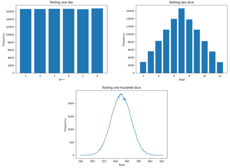
Consider a standard six-sided die. Every time you roll that die, an integer value results between 1 and 6, with equal probability. So, if you were to roll that die many, many times and then plot the frequency with which the different values occur, you will see a flat line; all six values arise with equal frequency.

Now, what happens when you roll a pair of dice and add them together? If you roll the pair of dice, integer values from 2 through 12 will result. If you were to roll the pair of dice many, many times and record their sum, what will the resulting distribution look like? You will not find a flat distribution; you will find that the distribution is peaked in the middle. Why? While only one combination of values yields a 2 (1 and 1), and only one combination yields a 12 (6 and 6), multiple combinations can yield a 7 (5 and 2, 2 and 5, 3 and 4, or 4 and 3). Note: if you have ever played Settlers of Catan, this may be familiar to you! This is why the 6 and 8 tiles are more desirable than the 2 or 12 tiles; the 6s and 8s occur more often.

This concept only amplifies as you add more die to the summation. That is, as you increase the number of random variables that enter your sum, the distribution of resulting values across trials will grow increasingly peaked in the middle. And, this property is not tied to the uniform distribution of a die; the same result will occur if you sum random variables drawn from any underlying distribution.