How to generate uniformly distributed points on the surface of the 3-d unit sphere?

Question

I am wondering how to generate uniformly distributed points on the surface of the 3-d unit sphere? Also after generating those points, what is the best way to visualize and check whether they are truly uniform on the surface $x^2+y^2+z^2=1$?

Answer 1

A standard method is to generate three standard normals and construct a unit vector from them. That is, when $X_i \sim N(0,1)$ and $\lambda^2 = X_1^2 + X_2^2 + X_3^2$, then $(X_1/\lambda, X_2/\lambda, X_3/\lambda)$ is uniformly distributed on the sphere. This method works well for $d$-dimensional spheres, too.

In 3D you can use rejection sampling: draw $X_i$ from a uniform$[-1,1]$ distribution until the length of $(X_1, X_2, X_3)$ is less than or equal to 1, then--just as with the preceding method--normalize the vector to unit length. The expected number of trials per spherical point equals $2^3/(4 \pi / 3)$ = 1.91. In higher dimensions the expected number of trials gets so large this rapidly becomes impracticable.

There are many ways to check uniformity. A neat way, although somewhat computationally intensive, is with Ripley's K function. The expected number of points within (3D Euclidean) distance $\rho$ of any location on the sphere is proportional to the area of the sphere within distance $\rho$, which equals $\pi\rho^2$. By computing all interpoint distances you can compare the data to this ideal.

General principles of constructing statistical graphics suggest a good way to make the comparison is to plot variance-stabilized residuals $e_i(d_{[i]} - e_i)$ against $i = 1, 2, \ldots, n(n-1)/2=m$ where $d_{[i]}$ is the $i^\text{th}$ smallest of the mutual distances and $e_i = 2\sqrt{i/m}$. The plot should be close to zero. (This approach is unconventional.)

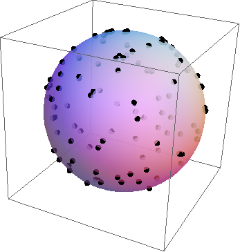
Here is a picture of 100 independent draws from a uniform spherical distribution obtained with the first method:

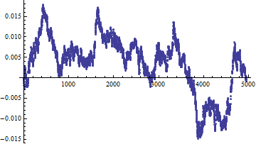
Here is the diagnostic plot of the distances:

The y scale suggests these values are all close to zero.

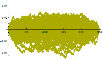
Here is the accumulation of 100 such plots to suggest what size deviations might actually be significant indicators of non-uniformity:

(These plots look an awful lot like Brownian bridges...there may be some interesting theoretical discoveries lurking here.)

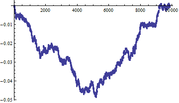
Finally, here is the diagnostic plot for a set of 100 uniform random points plus another 41 points uniformly distributed in the upper hemisphere only:

Relative to the uniform distribution, it shows a significant decrease in average interpoint distances out to a range of one hemisphere. That in itself is meaningless, but the useful information here is that something is non-uniform on the scale of one hemisphere. In effect, this plot readily detects that one hemisphere has a different density than the other. (A simpler chi-square test would do this with more power if you knew in advance which hemisphere to test out of the infinitely many possible ones.)

Answer 2

Here is some rather simple R code

n     <- 100000                  # large enough for meaningful tests
z     <- 2*runif(n) - 1          # uniform on [-1, 1]
theta <- 2*pi*runif(n) - pi      # uniform on [-pi, pi]
x     <- sin(theta)*sqrt(1-z^2)  # based on angle
y     <- cos(theta)*sqrt(1-z^2)     

It is very simple to see from the construction that $x^2+y^2 = 1- z^2$ and so $x^2+y^2+z^2=1$ but if it needs to be tested then

mean(x^2+y^2+z^2)  # should be 1
var(x^2+y^2+z^2)   # should be 0

and easy to test that each of $x$ and $y$ are uniformly distributed on $[-1,1]$ ($z$ obviously is) with

plot.ecdf(x)  # should be uniform on [-1, 1]
plot.ecdf(y)
plot.ecdf(z)

Clearly, given a value of $z$, $x$ and $y$ are uniformly distributed around a circle of radius $\sqrt{1-z^2}$ and this can be tested by looking at the distribution of the arctangent of their ratio. But since $z$ has the same marginal distribution as $x$ and as $y$, a similar statement is true for any pair, and this too can be tested.

plot.ecdf(atan2(x,y)) # should be uniform on [-pi, pi]
plot.ecdf(atan2(y,z))
plot.ecdf(atan2(z,x))

If still unconvinced, the next steps would be to look at some arbitrary 3-D rotation or how many points fell within a given solid angle, but that starts to get more complicated, and I think is unnecessary.

Answer 3

If you want to sample points uniformly distributed on the 3D sphere (i.e., the surface of a 3D ball), use a simple rejection, or the method of Marsaglia (Ann. Math. Statist., 43 (1972), pp. 645–646). For low dimensions, the rejection ratio is quite low.

If you want to generate random points from higher-dimensional spheres and balls, then it depends on the purpose and scale of the simulation. If you do not want to perform large simulations, use the method of Muller (Commun. ACM, 2 (1959), pp. 19–20) or its "ball" version (see the paper of Harman & Lacko cited above). That is:

to get a sample uniformly distributed on an n-sphere (surface) 1) generate X from n-dimensional standard normal distribution 2) divide each component of X by the Euclidean norm of X

to get a sample uniformly distributed on an n-ball (interior) 1) generate X from (n+2)-dimensional standard normal distribution 2) divide each component of X by the Euclidean norm of X and take only first n components

If you want to perform large simulations, then you should investigate more specialized methods. Upon request, I can send you the paper of Harman and Lacko on conditional distribution methods, which provides the classification and generalizations of some algorithms mentioned in this discussion. The contact is available at my website (http://www.iam.fmph.uniba.sk/ospm/Lacko)

If you want to check, whether yout points are truly uniform on the surface or interior of a ball, look at the marginals (all should by the same, because of the rotational invariance, the squared norm of a projected sample is beta distributed).

Answer 4

I had a similar problem (n-sphere) during my PhD and one of the local 'experts' suggested rejection sampling from a n-cube! This, of course, would have taken the age of the universe as I was looking at n in the order of hunderds.

The algorithm I ended up using is very simple and published in:

W.P. Petersen and A. Bernasconic Uniform sampling from an n-sphere: Isotropic method Technical Report, TR-97-06, Swiss Centre for Scientific Computing

I also have this paper in my bibliography that I havent looked at. You may find it useful.

Harman, R. & Lacko, V. On decompositional algorithms for uniform sampling from $n$-spheres and $n$-balls Journal of Multivariate Analysis, 2010

Answer 5

Here is the pseudocode:

1. $v \sim MultiVariateGaussian(\mu,\sigma I)$
2. $v = \frac{v}{ \| v \| }$

In pytorch:

v = MultivariateNormal(torch.zeros(10000), torch.eye(10000))
v = v/v.norm(2)

---

I don't understand this well enough but I've been told by whuber that:

v = torch.normal(torch.zeros(10000), torch.eye(10000))
v = v/v.norm(2)

is also correct i.e. sampling from a univariate normal for each coordinate.

Answer 6

I have had this problem before, and here is an alternative I found,

As for the distribution itself, the formula I found that works decently is to use polar coordinates (I actually use a variation of poler coordinates that developed), then convert to Cartesian coordinates.

The radius is of course the radius of the sphere on which you are plotting . Then you have the second value for angle on the flat plane, followed by the third value which is the angle above or below that plane.

To get a decent distribution, assume that U is a uniformly distributed random number, r is radius, a is the second polar coordinate, and b is the third polar coordinate,

a=U*360 b=U+U-1 then convert to cartesian via x=r*sin(b)sin(a) z=rsin(b)cos(a) y=rsin(b)

I recently found the following which is better mathematically speaking, a=2(pi)*U b=cos^-1(2U-1)

Not much different from my original formula actually, though mine is degrees vs radians.

This recent version supposedly can be used for hyperspheres, though no mention was made on how to achieve it.

Though I check the uniformity visually by the rather cheap method of making maps for Homeworld 2 and then "playing" those maps. In fact, because the maps are made with lua scripts, you can build your formula right into the map and thus check multiple samplings without ever leaving the game. Not scientific perhaps, but is a good method for visually seeing the the results.

Answer 7

My best guess would be to first generate a set of uniformly distributed points in 2 dimensional space and to then project those points onto the surface of a sphere using some sort of projection.

You will probably have to mix and match the way you generate the points with the way that you map them. In terms of the 2D point generationgeneration, I think that scrambled low-discrepancy sequences would be a good place to start (i.e. a scrambled Sobol sequence) since it usually produces points that are not "clumped together". I'm not as sure about which type of mapping to use, but Woflram popped up the Gnonomic projection... so maybe that could work?

MATLAB has a decent implementation of low discrepancy sequences which you can generate using q = sobolset(2) and scramble using q = scramble(q). There is also a mapping toolbox in MATLAB with a bunch of different projection functions you could use in case you did not want to code the mapping and graphics yourself.