29
$\begingroup$

I know that linear regression can be thought as "the line that is vertically closest to all the points":

enter image description here

But there is another way to see it, by visualizing the column space, as "the projection onto the space spanned by the columns of the coefficient matrix":

enter image description here

My question is: in these two interpretations, what happens when we use the penalized linear regression, like ridge regression and LASSO? What happens with the line in the first interpretation? And what happens with the projection in the second interpretation?

UPDATE: @JohnSmith in the comments brought up the fact that the penalty occurs in the space of the coefficients. Is there an interpretation in this space also?

$\endgroup$
2
  • 1
    $\begingroup$ I am not sure that it is possible to come up with such an interpretation. Simply because what you provided are images in the original space of features and responses. And penalized regression involves the space of coefficients, which is very different. $\endgroup$ Commented Jun 14, 2012 at 16:02
  • $\begingroup$ "the line vertically closest to all the points" ? One usually takes the sum of squares -- see the nice picture on Wikipedia Coefficient_of_determination. The sum of vertical distances is the L1 norm, which is less sensitive to outliers but much less common. $\endgroup$
    – denis
    Commented Jan 20, 2014 at 9:54

3 Answers 3

32
$\begingroup$

Sorry for my painting skills, I will try to give you the following intuition.

Let $f(\beta)$ be the objective function (for example, MSE in case of regression). Let's imagine the contour plot of this function in red (of course we paint it in the space of $\beta$, here for simplicity $\beta_1$ and $\beta_2$).

There is a minimum of this function, in the middle of the red circles. And this minimum gives us the non-penalized solution.

Now we add different objective $g(\beta)$ which contour plot is given in blue. Either LASSO regularizer or ridge regression regularizer. For LASSO $g(\beta) = \lambda (|\beta_1| + |\beta_2|)$, for ridge regression $g(\beta) = \lambda (\beta_1^2 + \beta_2^2)$ ($\lambda$ is a penalization parameter). Contour plots shows the area at which the function have the fixed values. So the larger $\lambda$ - the faster $g(x)$ growth, and the more "narrow" the contour plot is.

Now we have to find the minimum of the sum of this two objectives: $f(\beta) + g(\beta)$. And this is achieved when two contour plots meet each other.
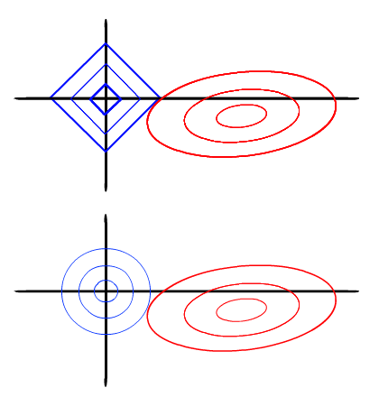
LASSO and Ridge regression

The larger penalty, the "more narrow" blue contours we get, and then the plots meet each other in a point closer to zero. An vise-versa: the smaller the penalty, the contours expand, and the intersection of blue and red plots comes closer to the center of the red circle (non-penalized solution).

And now follows an interesting thing that greatly explains to me the difference between ridge regression and LASSO: in case of LASSO two contour plots will probably meet where the corner of regularizer is ($\beta_1 = 0$ or $\beta_2 = 0$). In case of ridge regression that is almost never the case.

That's why LASSO gives us sparse solution, making some of parameters exactly equal $0$.

Hope that will explain some intuition about how penalized regression works in the space of parameters.

$\endgroup$
10
  • $\begingroup$ I think starting with a classical picture, as you've done, is a good start. To really understand this, I think it would be helpful to describe how the contours relate to the problem. In particular, we know in both cases, that the smaller we make our penalty, the closer we'll get to the OLS solution, and the larger it gets, the closer to a pure-intercept model we'll get. One question to ask is: How does this manifest itself in your figure? $\endgroup$
    – cardinal
    Commented Jun 15, 2012 at 14:37
  • $\begingroup$ By the way, your painting skills seem just fine. $\endgroup$
    – cardinal
    Commented Jun 15, 2012 at 14:41
  • $\begingroup$ Thanks for your comment! Everything is intuitively simple here: the larger penalty, the "more narrow" blue contours we get (and then the point two plots meet come closer to zero). An vise-versa: the smaller the penalty: the closer to the center of the red circle the plots will meet (OLS). $\endgroup$ Commented Jun 15, 2012 at 14:43
  • 2
    $\begingroup$ I updated the answer, introduced a more exact notation: $g(x)$ for the blue plots, $\lambda$ for the penalization paramater. Does that explain your concern better now? $\endgroup$ Commented Jun 15, 2012 at 15:07
  • 1
    $\begingroup$ Thanks for the clear illustration. I have read elsewhere that the minimum sum of the objectives occurs where they are tangent to each other. I get that if f(\beta)' = -g(\beta)' that would mean the derivative of the sum is zero which is a requirement for an extremum. Is this what is meant here by "when two contour plots meet each other"? $\endgroup$
    – odedbd
    Commented Jul 30, 2015 at 11:31
3
$\begingroup$

The intuition I have is the following: In the least-squares case, the hat matrix is an orthogonal projection thus idempotent. In the penalized case, the hat matrix is no longer idempotent. Actually, applying it infinitely many times, will shrink the coefficients to the origin. On the other hand, the coefficients still have to lie in the span of the predictors, so it is still a projection, albeit not orthogonal. The magnitude of the penalizing factor and the type of norm control the distance and direction of shrinkage towards the origin.

$\endgroup$
2
  • 1
    $\begingroup$ I can't see why it's not idempotent: if I project the vector in the space (even if it's not orthogonal projection), and I put a constraint in the coefficients, why would a new projection of this projected vector be different from the previous one? $\endgroup$
    – Lucas Reis
    Commented Jun 19, 2012 at 11:05
  • 1
    $\begingroup$ Intuitively: Say you are minimizing the penalized sum of squares a second time. The sum of squares at the second minimization is smaller than the sum of squares of the first minimization. The relative importance of the penalized coefficients' norm will increase, i.e., there is more to be gained by shrinking the coefficients some more. Ridge regression is a good example in which you have a nice closed form for the hat matrix and you can directly check if it is idempotent. $\endgroup$
    – JohnRos
    Commented Jun 19, 2012 at 19:30
1
$\begingroup$

Second image

The geometric interpretation in the second figure will look as following:

With OLS the observations are projected onto a surface spanned by the regressor variables and this finds the point in the plane that has the shortest distance to the observed vector $(y_1,y_2,y_3)$.

With ridge regression we do not look for a closest point in the entire plane but for a closest point that is inside a circle on the plane (or sphere in higher dimensions and other shape for different types of regression).

least squares vs regularized

Image from the question Why does regularization wreck orthogonality of predictions and residuals in linear regression?

First image

Regularisation will reduce the size of the parameters. So, the fitted line will have a smaller intercept and a smaller slope. In general this will mean that the line will be more flat and closer to the x-axis.

$\endgroup$

Your Answer

By clicking “Post Your Answer”, you agree to our terms of service and acknowledge you have read our privacy policy.

Not the answer you're looking for? Browse other questions tagged or ask your own question.