Relationship between Binomial and Beta distributions

Question

I'm more of a programmer than a statistician, so I hope this question isn't too naive.

It happens in sampling program executions at random times. If I take N=10 random-time samples of the program's state, I could see function Foo being executed on, for example, I=3 of those samples. I'm interested in what that tells me about the actual fraction of time F that Foo is in execution.

I understand that I is binomially distributed with mean F*N. I also know that, given I and N, F follows a beta distribution. In fact I've verified by program the relationship between those two distributions, which is

cdfBeta(I, N-I+1, F) + cdfBinomial(N, F, I-1) = 1

The problem is I don't have an intuitive feel for the relationship. I can't "picture" why it works.

EDIT: All the answers were challenging, especially @whuber's, which I still need to grok, but bringing in order statistics was very helpful. Nevertheless I've realized I should have asked a more basic question: Given I and N, what is the distribution for F? Everyone has pointed out that it's Beta, which I knew. I finally figured out from Wikipedia (Conjugate prior) that it appears to be Beta(I+1, N-I+1). After exploring it with a program, it appears to be the right answer. So, I would like to know if I'm wrong. And, I'm still confused about the relationship between the two cdfs shown above, why they sum to 1, and if they even have anything to do with what I really wanted to know.

Answer 1

Consider the order statistics $x_{[0]} \le x_{[1]} \le \cdots \le x_{[n]}$ of $n+1$ independent draws from a uniform distribution. Because uniform order statistics have Beta distributions, the chance that $x_{[k]}$ does not exceed $p$ is given by the Beta integral

$$\Pr[x_{[k]} \le p] = \frac{1}{B(k+1, n-k+1)} \int_0^p{x^k(1-x)^{n-k}dx}.$$

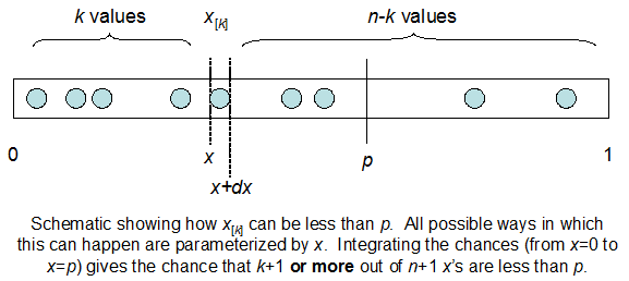
(Why is this? Here is a non-rigorous but memorable demonstration. The chance that $x_{[k]}$ lies between $p$ and $p + dp$ is the chance that out of $n+1$ uniform values, $k$ of them lie between $0$ and $p$, at least one of them lies between $p$ and $p + dp$, and the remainder lie between $p + dp$ and $1$. To first order in the infinitesimal $dp$ we only need to consider the case where exactly one value (namely, $x_{[k]}$ itself) lies between $p$ and $p + dp$ and therefore $n - k$ values exceed $p + dp$. Because all values are independent and uniform, this probability is proportional to $p^k (dp) (1 - p - dp)^{n-k}$. To first order in $dp$ this equals $p^k(1-p)^{n-k}dp$, precisely the integrand of the Beta distribution. The term $\frac{1}{B(k+1, n-k+1)}$ can be computed directly from this argument as the multinomial coefficient ${n+1}\choose{k,1, n-k}$ or derived indirectly as the normalizing constant of the integral.)

By definition, the event $x_{[k]} \le p$ is that the $k+1^\text{st}$ value does not exceed $p$. Equivalently, at least $k+1$ of the values do not exceed $p$: this simple (and I hope obvious) assertion provides the intuition you seek. The probability of the equivalent statement is given by the Binomial distribution,

$$\Pr[\text{at least }k+1\text{ of the }x_i \le p] = \sum_{j=k+1}^{n+1}{{n+1}\choose{j}} p^j (1-p)^{n+1-j}.$$

In summary, the Beta integral breaks the calculation of an event into a series of calculations: finding at least $k+1$ values in the range $[0, p]$, whose probability we normally would compute with a Binomial cdf, is broken down into mutually exclusive cases where exactly $k$ values are in the range $[0, x]$ and 1 value is in the range $[x, x+dx]$ for all possible $x$, $0 \le x \lt p$, and $dx$ is an infinitesimal length. Summing over all such "windows" $[x, x+dx]$--that is, integrating--must give the same probability as the Binomial cdf.

Answer 2

Look at the pdf of Binomial as a function of $x$: $$f(x) = {n\choose{x}}p^{x}(1-p)^{n-x}$$ and the pdf of Beta as a function of $p$: $$g(p)=\frac{\Gamma(a+b)}{\Gamma(a)\Gamma(b)}p^{a-1}(1-p)^{b-1}$$ You probably can see that with an appropriate (integer) choice for $a$ and $b$ these are the same. As far as I can tell, that's all there is to this relationship: the way $p$ enters into the binomial pdf just happens to be called a Beta distribution.

Answer 3

As you noted, the Beta distribution describes the distribution of the trial probability parameter $F$, while the binomial distribution describes the distribution of the outcome parameter $I$. Rewriting your question, what you asked about was why $$P(F \le \frac {i+1} n)+P(I \le fn-1)=1$$ $$P(Fn \le i+1)+P(I+1 \le fn)=1$$ $$P(Fn \le i+1)=P(fn<I+1)$$ That is, the likelihood that the observation plus one is greater than the expectation of the observation is the same as the likelihood that the observation plus one is greater than the expectation of the observation.

I admit that this may not help intuit the original formulation of the problem, but maybe it helps to at least see how the two distributions use the same underlying model of repeated Bernoulli trials to describe the behavior of different parameters.

Answer 4

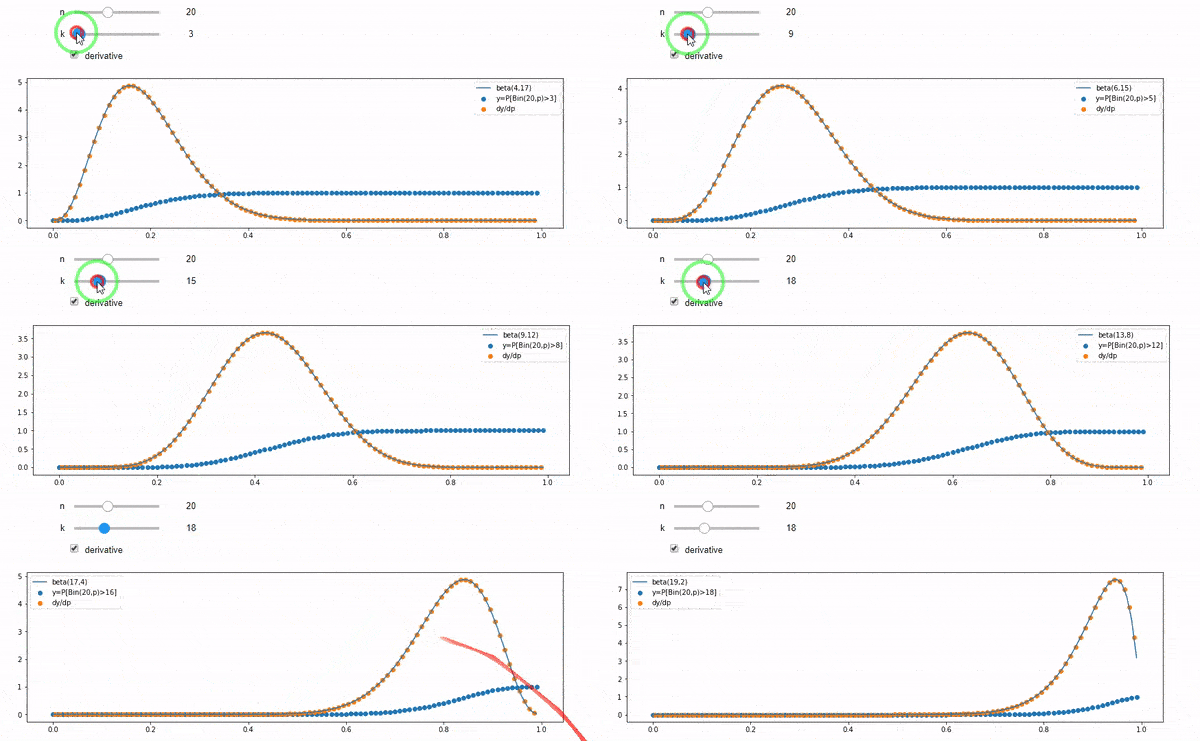
Summary: It is often said that Beta distribution is a distribution on distributions! But what is means?

It essentially means that you may fix $n,k$ and think of $\mathbb P[Bin(n,p)\geqslant k]$ as a function of $p$. What the calculation below says is that the value of $\mathbb P[Bin(n,p)\geqslant k]$ increases from $0$ to $1$ when you tune $p$ from $0$ to $1$. The increasing rate at each $p$ is exactly $\beta(k,n-k+1)$ at that $p$.

---

Let $Bin(n,p)$ denote a Binomial random variable with $n$ samples and the probability of success $p$. Using basic algebra we have

$$\frac d{dp}\mathbb P[Bin(n,p)=i]=n\Big(\mathbb P[Bin(n-1,p)=i-1]-\mathbb P[Bin(n-1,p)=i]\Big).$$

It has also some nice combinatorial proof, think of it as an exercise!

So, we have:

$$\frac d{dp}\mathbb P[Bin(n,p)\geqslant k]=\frac d{dp}\sum_{i=k}^{n}\mathbb P[Bin(n,p)=i]=n\Big(\sum_{i=k}^{n}\mathbb P[Bin(n-1,p)=i-1]-\mathbb P[Bin(n-1,p)=i]\Big)$$ which is a telescoping series and can be simplified as

$$\frac d{dp}\mathbb P[Bin(n,p)\geqslant k]=n\mathbb P[Bin(n-1,p)=k-1]=\frac{n!}{(k-1)!(n-k)!}p^{k-1}(1-p)^{n-k}=\beta(k,n-k+1).$$

---

Remark To see an interactive version of the plot look at this. You may download the notebook or just use the Binder link.

Answer 5

In Bayesian land, the Beta distribution is the conjugate prior for the p parameter of the Binomial distribution.

Answer 6

Can't comment on other answers, so i have to create my own answer.

Posterior = C * Likelihood * Prior (C is a constant that makes Posterior integrated to 1)

Given a model that uses Binomial distribution for likelihood, and Beta distribution for Prior. The product of the two which generates the Posterior is also a Beta distribution. Since the Prior and Posterior are both Beta, and thus they are conjugate distributions. the Prior (a Beta) is called conjugate prior for the likelihood (a Binomial). For example, if you multiply a Beta with a Normal, the Posterior is no longer a Beta. In summary, Beta and Binomial are two distributions that are frequently used in Bayesian inference. Beta is Conjugate Prior of Binomial, but the two distributions are not a subset or superset of the other.

The key idea of Bayesian inference is we are treating the parameter p as a random variable that ranges from [0,1] which is contrary to frequentist inference approach where we are treating parameter p as fixed. If you look closely to the properties of Beta distribution, you will see its Mean and Mode are solely determined by $\alpha$ and $\beta$ irrelevant to the parameter p . This, coupled with its flexibility, is why Beta is usually used as a Prior.

Answer 7

Here is an intuitive explanation that works for me:

$Binomial(n, p)$:
When repeating a Bernoulli trial with $p$ probability $n$ times. The chance of exactly $k$ successes is: $$Binomial_\mathit{pmf}(\pmb{k}, n, p) = {n\choose \pmb{k}} p^{\pmb{k}} (1-p)^{n-\pmb{k}}$$

$Beta(n, k)^*$:
For a fixed $n$ and $k$, given probability $p$, calculate the probability, $p'$, of getting $k$ in the former experiment. Then multiply this $p'$ by $n+1$ to get $k'$, the most probable (interpolated) outcome if we have done the experiment with $p'$ (conceptually this is like the mode of $Binomial(n, p')$, only it allowes for non-integer values):

$$Beta_\mathit{pdf}(\pmb{p}, n, k) = \underbrace{(n+1) \overbrace{{n \choose k} \pmb{p}^k (1-\pmb{p})^{n-k}}^{p'=Binomial_\mathit{pmf}(k, n, \pmb{p})}}_{k' \approx mode(Binomial(n, p'))}$$

$\small{*}$ I'm using ${n \choose k}$ to emphasize the similarity with the $Binomial$. To get the actual $Beta$ function we need to replace $\cdot!$ with $\Gamma(\cdot+1)$, which interpolates the factorial for non-integer values.

Note 1: If $p$ is close to $k/n$, k′ is larger.

Note 2: If the parameter $n$ is larger we are more certain of the result (the concentration is higher).

Note 3: The get the common formulation for the $Beta(\alpha,\beta)$ function:
$$k \to \alpha - 1$$ $$n \to \alpha + \beta- 2$$

Note 4: When replacing $\cdot!$ by $\Gamma(\cdot+1)$, $Beta(n, k)$ is actually defined for real-valued $n$ and $k$, with ranges $n > k - 1$ and $k > -1$. We can think of things like -0.3 successes out of -1.1 Bernoulli trials as interpolations from the integer $0 \le k \le n$ cases.

Note 5: $Beta(n=0, k=0) \equiv Uniform(0,1)$

Note 6: $\int_0^1(n+1){n\choose k} p^k (1-p)^{n-k} \,dp = 1$