Difference between splines from different packages (mgcv, rms etc.)

Question

I recently came across the mgcv package and the great potentiality of GAM. One - maybe naive - question is what is the overall difference (if there is any which is significant) with the gam() function of the mgcv package, compared for example with the use of restricted cubic splines in the rms package.

Is there something big that I am missing?

Answer 1

The main difference is the choice of knots and penalization. To start, let's focus on cubic splines for x, y data.*

I find it useful to start from the extreme situation, an interpolating spline that connects all data points with a smooth curve. Then each x-axis value is a knot at which two cubic functions interpolating on either side of the knot agree in their values (and with the corresponding y value) and in their first and second derivatives. That can fit the data at hand perfectly but at the cost of a very "wiggly" curve and probable overfitting that won't generalize well to new data.

The different approaches can be thought of as different ways to avoid that overfitting.

A cubic smoothing spline might keep the original knot locations along the x-axis while penalizing the roughness of the curve in terms of its integrated squared second derivative. An optimal penalty can be chosen by (restricted) marginal likelihood or generalized cross-validation.

That Wikipedia entry outlines other methods, including regression splines and penalized splines:

Regression splines. In this method, the data is fitted to a set of spline basis functions with a reduced set of knots, typically by least squares. No roughness penalty is used...

Penalized splines. This combines the reduced knots of regression splines, with the roughness penalty of smoothing splines.

Thin plate splines and Elastic maps method for manifold learning. This method combines the least squares penalty for approximation error with the bending and stretching penalty of the approximating manifold and uses the coarse discretization of the optimization problem.

In this terminology, the mgcv package has a major focus on smoothing/penalization methods, with thin-plate splines as a default, although it can accommodate unpenalized regression splines. (The help pages for that package don't restrict the term "regression splines" to unpenalized methods.)

A simple implementation of penalized splines is seen in the pspline() function in the survival package, which sets up a small set of evenly spaced symmetric basis functions that span the x-axis data range. The corresponding coefficients are then penalized automatically when fitting coxph or survreg survival models.

The ns() and rcs() functions implement "natural" cubic regression splines, restricted to be linear beyond the outermost knots. By your choice of the number of knots, you thus specify the number of degrees of freedom to be used in the fit. There is no inherent penalization beyond the choice of numbers of knots.

Therneau and Grambsch, in Modeling Survival Data: Extending the Cox Model discuss regression splines in Section 5.4 and smoothing splines in Section 5.5, without massive mathematical detail about spline basis functions that can become confusing. They put one difference between them this way:

One issue with regression splines is the arbitrary choice of control point (knot) locations. Are the default quantiles good values, would the curve change significantly if other knot locations were selected, or can knot position be optimized? For a data set that contains a sudden feature, such as a changepoint, the choice of particular knot locations may either enhance or mask the feature.

An alternative to the regression spline is a smoothing spline.

That said, their pspline() function spaces a limited number of basis functions evenly across the x-axis value range, without regard to the distribution of x values. See Section 5.8.3 of their book. One might consider that a different "arbitrary choice."

Furthermore, regression splines allow you to pre-specify how many degrees of freedom to devote to the modeled predictor. That's an advantage with Harrell's approach to Regression Modeling Strategies, in which such explicit choices early in modeling are key. With penalization methods, one typically lets the data determine how many degrees of freedom to use up. Regression splines work well in practice with typical data, when you don't need the highly specialized types of fits provided by mgcv for things like geospatial data.

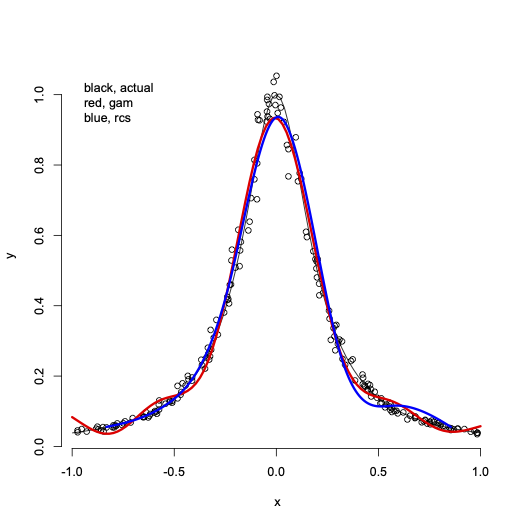
Here's a particular comparison of rcs() and gam() fitting of data generated from the Runge function; code is below.

The gam() fit devoted 8.95 degrees of freedom (df) to the penalized fit, plus the intercept for 9.95 df total. The corresponding df used by the ols() fit with an rcs(x,7) term were 6 for x and 7 df total.

Whichever choice you make, don't just accept default parameter settings blindly; not to choose is to choose, and you should understand the choices you are (even implicitly) making about your spline approximation. For example, the gam() fit above used the default bs=tp (thin-plate spline) setting for the smoothing basis, which "do not have ‘knots’ (at least not in any conventional sense): a truncated eigen-decomposition is used to achieve the rank reduction." With this size data set, the rcs(x,7) term led to outer knots at the 0.05 and 0.95 quantiles of x values, with 5 interior knots "equally spaced between these on the quantile scale." (Emphasis added.) Read the help pages carefully.

This site has many posts on these types of splines. Frank Harrell, author of the rms package, often discusses regression splines. Gavin Simpson, author of the gratia package that helps to visualize mgcv models, often discusses GAM. Searches here for posts by those reputable sources will provide much for further study.

Code for the figure:

runge <- function(x) {1/(1+25*x^2)}
set.seed(1)
xvals <- runif(200,min=-1,max=1)
yvals <- exp(log(runge(xvals))+log(rlnorm(200,sdlog=0.075))) ## add some multiplicative error
dfspl <- data.frame(x=xvals,y=yvals)
library(rms)
library(mgcv)
ddspl <- datadist(dfspl)
options(datadist="ddspl")
olsFit7 <- ols(y~rcs(x,7),data=dfspl) ## default is 5 knots, used 7
gamFit <- gam(y~s(x),data=dfspl) ## use defaults
plot(y~x,data=dfspl,bty="n")
curve(runge(x),from=-1,to=1,add=TRUE)
lines(seq(-1,1,length.out=100),predict(gamFit,newdata=data.frame(x=seq(-1,1,length.out=100))),col="red",lwd=3)
lines(Predict(olsFit7),col="blue",lwd=3)
legend("topleft",legend="black, actual\nred, gam\nblue, rcs",bty="n")

## to see an interpolating spline for these data, run
## isplFit <- splines::interpSpline(y~x,dfspl); plot(predict(isplFit,seq(-1,1,length.out=500)),type="l")

---

*There can be different choices of the basis functions used to construct the cubic splines, but as comments note those choices are somewhat arbitrary and should give similar results in practice. Also, a default spline in the mgcv package doesn't involve knots in the usual sense at all, as the answer eventually notes.