External clustering criteria either don’t rely on group correspondence between the being compared partitions U and V, or the correspondence between their groups is somehow determined implicitly by the very formula of the criterion. Typical usage example is a comparison among clusterings or between a done clustering and some classification. This answer will confine itself to mutually exclusive groups/clusters. The two being compared partitions U and V are two categorical variables with some arbitrary codings. (The answer is based on the description document for my SPSS macro !KO_cluagree found on my web-page in the collection "Compare partitions".)
There are two main types of measures: measures based on co-membership confusion matrix and measures based on frequency cross-tabulation of objects.
Co-membership confusion matrix measures aka object pairs measures
Let there be N objects and two being compared partitions into groups, partition U and partition V. All possible pairs of objects get considered and the following 2x2 frequency table (co-membership confusion matrix) counting pairs is filled in:

Pairs sum a is the ground of similarity between U and V, and pairs sum d can be the ground of similarity in some measures; b and c attenuate similarity.
The measures of similarity between partitions U and V can be symmetric or asymmetric. A symmetric measure will not change value if U (confusion matrix rows) and V (its columns) swap their places, i.e., the table gets transposed. An asymmetric measure will change value after the table is transposed. When a measure is asymmetric but the roles of two partitions are symmetric (two alternative clusterings), we usually come to average/combine two values; but if the roles are asymmetric (a clustering vs reference partition), we may leave and interpret both values according to their math meaning. $^1$
Some most used pairs measures. They are symmetric except where remarked; and similarities vary in [0,1], except where remarked.
Dice similarity aka F1 or F measure.
$DICE= 2a/(2a+b+c)=2P \cdot R/(P+R)$
where
$P=a/(a+c)$ is called co-membership precision, and
$R=a/(a+b)$ is called co-membership recall.
DICE (F measure) is the harmonic mean of recall R and precision P, which, in return, can be called the two “asymmetric versions” of the F measure.
Ochiai similarity aka Folkes–Mallows is the geometric mean of recall R and precision P. (So R and P can be seen as its asymmetric versions, too.)
$OCHIAI= a/\sqrt{(a+b)(a+c)} = \sqrt{P \cdot R}$
Kulczynski 2 similarity is the arithmetic mean of recall R and precision P. (So R and P can be seen as its asymmetric versions, too.)
$KULCZ2=(\frac{a}{a+b} + \frac{a}{a+c}) / 2 = (P+R)/2$
Jaccard similarity
$JACCARD=a/(a+b+c)$
Sokal-Sneath 2 similarity
$SS2=a/(a+2(b+c))$
Sokal-Sneath 1 similarity
$SS1=2(a+d)/(2(a+d)+b+c)$
Rand aka Simple matching similarity
$RAND=(a+d)/(a+d+b+c)$
Adjusted Rand similarity is RAND normalized in a stochastic sense under the assumption of hypergeometric distribution. The upper bound of ARAND for the observed pair of partitions equals 1 (if the number of groups is equal in the partitions), and the index is close to zero if both partitions of the objects into groups are independent and random (only group sizes are fixed). ARAND can take on negative values.
$ARAND=2(ad-bc)/((a+b)(d+b)+(a+c)(d+c))$
This measure is identical to Cohen’s kappa for the 2×2 table.
Russel–Rao similarity
$RR=a/(a+d+b+c)$
Rogers–Tanimoto similarity
$RT=(a+d)/(a+d+2(b+c))$
Phi correlation similarity aka normalized Hubert Г statistic. This is the Pearson correlation in situation of binary data. It can vary in the range from -1 to 1.
$PHI=(ad-bc)/ \sqrt{(a+b)(a+c)(b+d)(c+d)}$
Dispersion similarity. Can vary in the range from -1 to 1.
$DISPER=(ad-bc)/(a+d+b+c)^2$
squared Euclidean distance aka Hamming distance dissimilarity. It is a metric distance, and is linearly equivalent to 1-RAND. 2SEUCLID is known as Mirkin distance.
$SEUCLID=b+c$
McNemar distance dissimilarity. This is the square root of McNemar’s test statistic.
$MN=|b-c|/\sqrt{b+c}$
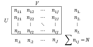
Frequency cross-tabulation of objects measures
Let there be N objects and two being compared partitions into groups, partition U (with groups 1, 2,…, I) and partition V (with groups 1, 2,…, J). We have the cross-tabulation:

The following cross-tabulation measures to compare clusterings are often used. Most are similarities. Some can have asymmetric versions. (What was said about asymmetric measures earlier holds to these too.)
Overlap similarity aka Purity, asymmetric measure:
$OVL_{UV}= \frac{1}{N} \sum_i^I \max_j^J n_{ij}$ and $OVL_{VU}= \frac{1}{N} \sum_j^J \max_i^I n_{ij}$
Its symmetric version: $OVL=(OVL_{UV}+OVL_{VU})/2$
appears to be a linear equivalent to 1-(Van Dongen Overlap distance). 1-OVL is a metric distance.
F Clustering Accuracy similarity, more sophisticated measure of overlap than OVL, accounting together for notions of “homogeneity” and “completeness”. (Perfectly homogeneous relation of V to U is when a group from V contains objects only of one group from U. Perfectly complete relation of V to U is when a group from V contains all objects of some group from U.) FCA is asymmetric:
$FCA_{UV}= \frac{1}{N} \sum_i^I n_{i.} \max_j^J F_{ij}$ and $FCA_{VU}= \frac{1}{N} \sum_j^J n_{.j} \max_i^I F_{ij}$
where $F_{ij}$ is cell F1 measure, equal to the harmonic mean:
$F_{ij}= 2R_{ij} \cdot P_{ij}/(R_{ij}+P_{ij}) = 2n_{ij}⁄(n_{i.}+n_{.j})$
$R_{ij}$ (recall) $=n_{ij}/n_{i.}$ and $P_{ij}$ (precision) $=n_{ij}/n_{.j}$
Symmetric version of FCA: $FCA= (FCA_{UV}+FCA_{VU})/2$
Mutual Information similarity, an entropic measure.
$H(U)=-\sum_i^I \frac{n_{i.}}{N} \ln \frac{n_{i.}}{N}$ is the entropy in partition U
$H(V)=-\sum_j^J \frac{n_{.j}}{N} \ln \frac{n_{.j}}{N}$ is the entropy in partition V
$H(U\&V)=-\sum_{i,j}^{IJ} \frac{n_{ij}}{N} \ln \frac{n_{ij}}{N}$ is the joint entropy of U and V
Then
$MI=H(U)+H(V)-H(U\&V)$
Variation of Information distance is MI translated into the metric distance by formula:
$VI=H(U)+H(V)-2MI$
Normalized Mutual Information similarity is MI normalized so that the possible range of the measure for the two given partitions U and V be from 0 to 1:
$NMI=MI/MI_{UpperBound}$
where upper bound, $MI_{UpperBound}$, can be chosen to be equal to:
$\max(H(U),H(V))$ (most often) or $\min(H(U),H(V))$ or $(H(U)+H(V))/2$ or $\sqrt{H(U)H(V)}$
Adjusted Mutual Information similarity is MI normalized in a stochastic sense. Its upper bound for the observed pair of partitions equals 1 (as in NMI), but AMI is close to zero in case both partitions into groups are purely random (only group sizes are fixed). AMI can take on negative values.
$AMI= \frac{MI-E(MI)}{MI_{UpperBound}-E(MI)}$
where $MI_{UpperBound}$ is defined as in NMI, while $E(MI)$ is the expected magnitude of MI when U and V are two independent, random disposition of objects into groups (group sizes are set there and there).
$E(MI)= \sum_{i,j}^{IJ} \sum_{x=\max(n_{i.}+n_{.j}-N,1)}^{\min(n_{i.},n_{.j})} \frac{x}{N} \ln (\frac{Nx}{n_{i.}n_{.j}}) \frac { (n_{i.}! n_{.j}! (N-n_{i.})! (N-n_{.j})! } {N! x! (n_{i.}-x)! (n_{.j}-x)! (N-n_{i.}-n_{.j}+x)!}$
(in this formula x is integer running over values “from” and “to”).
Homogeneity&Completeness V similarity, an entropic measure accounting for both notions “homogeneity” and “completeness” (see FCA above, for comparison), which it formulates as follows:
$h$ (homogeneity) $=1-H(U|V)/H(U)$, and with $H(U)=0$, $h=1$
$c$ (completeness) $=1-H(V|U)/H(V)$, and with $H(V)=0$, $c=1$
where the conditional entropies (see measure MI earlier):
$H(U|V)= H(U\&V)-H(V)$ and $H(V|U)= H(U\&V)-H(U)$
Harmonic mean of $h$ and $c$, a symmetric measure, is HCV:
$HCV=2hc/(h+c)$
$c$ and $h$ could be interpreted as asymmetric verions of HCV:
$HCV_{UV}=c$ and $HCV_{VU}=h$
Using classification comparison measures.
If you arrive at a definite conclusion which cluster in partition U corresponts to which cluster in partition V, in the sense it is as if a priori the same class, then you can see the task as the task of comparing classifications rather than clusterings, and use classification agreement indices. The one-to-one matching between U partition clusters and V partition clusters can sometimes be established immediately from contemplating the frequency cross-tabulation. When, not, try to use a matching algorithm such as Hungarian or a greedy matching. You might prefer to establish matches based on raw frequencies or maybe based on frequency residuals or on cell F measures. (My SPSS macro !KO_grmatch does the job of empirical matching of groups between partitions.)
Literature:
- Wagner, S., Wagner, D. Comparing clusterings - an overview // A manuscript: Univ., Fak. für Informatik, January 12, 2007.
- Vinh, N.X., Epps, J., Bailey, J. Information theoretic measures for clusterings comparison: variants, properties, normalization and correction for chance // Journal of Machine Learning Research, 2010, 11, 2837-2854.
- Vinh, N.X., Epps, J., Bailey, J. Information theoretic measures for clusterings comparison: is a correction for chance necessary? // Proceedings of the 26th International Conference on Machine Learning. Montreal, Canada, 2009.
- Rosenberg, A., Hirschberg, J. V-measure: a conditional entropy-based external cluster evaluation measure // Proceedings of the 2007 Joint Conference on Empirical Methods in Natural Language Processing and Computational Natural Language Learning. Prague, June 2007, 410–420.
- Romano, S. et al. Adjusting for chance clustering comparison measures // Journal of Machine Learning Research, 2016, 17, 1–32.
- Meila, M. Comparing clusterings – an information based distance // Journal of Multivariate Analysis, 2007, 98, 873–895.
- Desgraupes, B. Clustering indices // Package clusterCrit for R, April 2013.
- Rendon, E. et al. Internal versus external cluster validation indexes // International Journal of Computers and Communications, 2011, 1 (1), 27–34.
- Halkidi, M., Batistakis, Y., Vazirgiannis, M. On clustering validation techniques // Journal of Intelligent Information Systems, 2001, 17 (2/3), 107–145.
$^1$ A decision schema around the issue of asymmetric agreement indices. Indices can be symmetric or asymmetric mathematically and partitions can be symmetric or asymmetric positionally. Positionally symmetric partitions is when we're just comparing two alternative partitions. Positionally asymmetric partitions is when one of the two is "reference" and the other is "experimental" - different roles. Then...
If the index is symmetric and the roles are symmetric, then no problem. If the index is symmetric and the roles are asymmetric, we say: the given symmetric index serves the asymmetric roles (like, say, correlation coefficient is still a valid index in a cause-response relationship).
If the index is asymmetric and the roles are symmetric, then, in case of comparison of clustering partitions (i.e., no knowledge of labels is used) we treat the index asymmetry as a mere inconvenience and average/combine the two values (if the action defensible). But in case of comparison of classification partitions (knowledge of labels is used) we refuse the symmetry of roles and move to the situation where one partition is declared "reference" and the other "experimental".
If the index is asymmetric and the roles are asymmetric, then, in case of comparison of clustering partitions we may accept and interpret both distinct values of the index (plus possibly average/combine them into one). In case of comparison of classification partitions we interpret only one of the two values of the index, based on "who is who" in the partitions pair.


