Why is the x-axis labeling irregular in the plot.zph function?

Question

I am using the survival package in R to run cox proportional hazards models. My question is about the plot.zph function.

This code

plot(zph[1], lwd = 2) +
  abline(0, 0, col = 1, lty = 3, lwd = 2) +
  abline(
    h = cox.ph.mod$coef[1],
    col = 3,
    lwd = 2,
    lty = 2
)

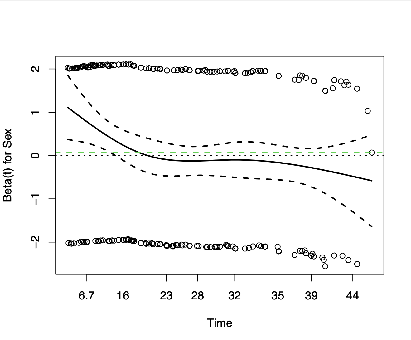
produces this plot:

My question is just about the irregular spacing of the x-axis. The tick marks are not evenly spaced, the labeling is irregular, and the distance between tick marks seems off. For example the space between 32 and 35 appears larger than the space between 35 and 39. This doesn't seem to be just a me problem; the plots in this tutorial seem to have the same issue: http://www.sthda.com/english/wiki/cox-model-assumptions

I'm assuming this does not severely impact the interpretation of the plot, but I am curious a) why this is happening, b) if it's a problem or if it's by design, and c) if it impacts interpretation in any way.

Thanks!

---

Answer 1

This is by design. The transform argument to cox.zph() allows different transformations of the time axis. This is discussed in Chapter 6 of Therneau and Grambsch.

The default Kaplan-Meier ("km") choice transforms time to correspond to probabilities of survival.* You can choose instead to space evenly by observation times ("rank"), use the original time scale ("identity"), its log transformation ("log"), or any specific transformation you wish.

The Kaplan-Meier transformation is the default because it's less sensitive to censoring patterns than the rank transformation and it tends to spread residuals (calculated at event times) more evenly across the plot from left to right. For example, in a frequent situation with just a few individuals having events at late times, with an "identity" transformation you would have a lot of events bunched together at early times and events at very late times would visually overwhelm the display of the smoothed curve.

The transformations can affect the p-values returned by the test, as the test is effectively for a trend in scaled Schoenfeld residuals with respect to the transformed time axis. Therneau and Grambsch show how different choices for time transformation correspond to different tests that have been proposed for proportional hazards.

---

*"Consider a plot of t versus (1 - KM(t-)), and replace each time point by its vertical position on the plot." Page 136, Therneau and Grambsch.