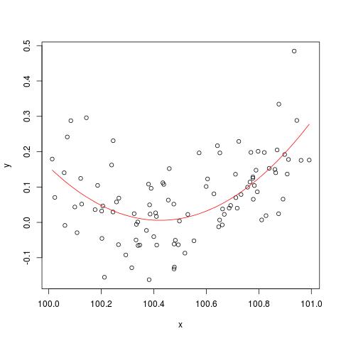
To illustrate the numerical stability issue mentioned by @cbeleites, here is an example from Simon Wood on how to "break" lm(). First we'll generate some simple data and fit a simple quadratic curve.

set.seed(1); n <- 100
xx <- sort(runif(n))
y <- .2*(xx-.5)+(xx-.5)^2 + rnorm(n)*.1
x <- xx+100
b <- lm(y ~ x+I(x^2))

plot(x,y)
lines(x, predict(b), col='red')

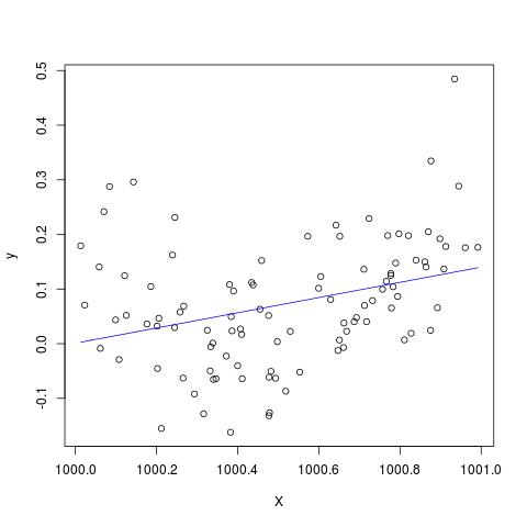
But if we add 900 to X, then the result should be pretty much the same except shifted to the right, no? Unfortunately not...

X <- x + 900
B <- lm(y ~ X+I(X^2))
plot(X,y)
lines(X, predict(B), col='blue')

Other algorithms can of course be "broken" in different ways with different examples.

To illustrate the numerical stability issue mentioned by @cbeleites, here is an example from Simon Wood on how to "break" lm(). First we'll generate some simple data and fit a simple quadratic curve.

set.seed(1); n <- 100
xx <- sort(runif(n))
y <- .2*(xx-.5)+(xx-.5)^2 + rnorm(n)*.1
x <- xx+100
b <- lm(y ~ x+I(x^2))

plot(x,y)
lines(x, predict(b), col='red')

But if we add 900 to X, then the result should be pretty much the same except shifted to the right, no? Unfortunately not...

X <- x + 900
B <- lm(y ~ X+I(X^2))
plot(X,y)
lines(X, predict(B), col='blue')

Edit to add to the comment by @Scortchi - if we look at the object returned by lm() we see that the quadratic term has not been estimated and is shown as NA.

> B
Call:
lm(formula = y ~ X + I(X^2))

Coefficients:
(Intercept)            X       I(X^2)  
  -139.3927       0.1394           NA  

And indeed as suggested by @Scortchi, if we look at the model matrix and try to solve directly, it "breaks".

> X <- model.matrix(b) ## get same model matrix used above
> beta.hat <- solve(t(X)%*%X,t(X)%*%y) ## direct solution of ‘normal equations’
Error in solve.default(t(X) %*% X, t(X) %*% y) : 
  system is computationally singular: reciprocal condition number = 3.9864e-19

However, lm() does not give me any warning or error message other than the NAs on the I(X^2) line of summary(B) in R-3.1.1. Other algorithms can of course be "broken" in different ways with different examples.