deleted 5 characters in body
Source Link
Glen_b
  • 290.4k
  • 37
  • 652
  • 1.1k

In an unpenalized regression, you can often get a ridge* in parameter space, where many different values along the ridge all do as well or nearly as well on the least squares criterion.

* (at least, it's a ridge in the likelihood function -- they're actually valleys$ in the RSS criterion, but I'll continue to call it a ridge, as this seems to be conventional -- or even, as Alexis points out in comments, I could call that a thalweg, being the valley's counterpart of a ridge)

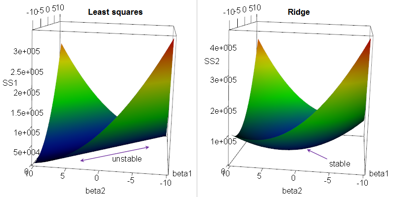
In the presence of a ridge in the least squares criterion in parameter space, the penalty you get with ridge regression gets rid of those ridges by pushing the criterion up as the parameters head away from the origin:

enter image description here
[Clearer image]

In the first plot, a large change in parameter values (along the ridge) produces a miniscule change in the RSS criterion. This can cause numerical instability; it's very sensitive to small changes (e.g. a tiny change in a data value, even truncation or rounding error). The parameter estimates are almost perfectly correlated. You may get parameter estimates that are very large in magnitude.

By contrast, by lifting up the thing that ridge regression minimizes (by adding the $L_2$ penalty) when the parameters are far from 0, small changes in conditions (such as a little rounding or truncation error) can't produce gigantic changes in the resulting estimates. The penalty term results in shrinkage toward 0 (resulting in some bias). A small amount of bias can buy a substantial improvement in the variance (by eliminating that ridge).

The uncertainty of the estimates are reduced (the standard errors are inversely related to the second derivative, which is made larger by the penalty).

Correlation in parameter estimates is reduced. You now won't get parameter estimates that are very large in magnitude if the RSS for small parameters would fit just about as wellnot be much worse.

In an unpenalized regression, you can often get a ridge* in parameter space, where many different values along the ridge all do as well or nearly as well on the least squares criterion.

* (at least, it's a ridge in the likelihood function -- they're actually valleys$ in the RSS criterion, but I'll continue to call it a ridge, as this seems to be conventional -- or even, as Alexis points out in comments, I could call that a thalweg, being the valley's counterpart of a ridge)

In the presence of a ridge in the least squares criterion in parameter space, the penalty you get with ridge regression gets rid of those ridges by pushing the criterion up as the parameters head away from the origin:

enter image description here
[Clearer image]

In the first plot, a large change in parameter values (along the ridge) produces a miniscule change in the RSS criterion. This can cause numerical instability; it's very sensitive to small changes (e.g. a tiny change in a data value, even truncation or rounding error). The parameter estimates are almost perfectly correlated. You may get parameter estimates that are very large in magnitude.

By contrast, by lifting up the thing that ridge regression minimizes (by adding the $L_2$ penalty) when the parameters are far from 0, small changes in conditions (such as a little rounding or truncation error) can't produce gigantic changes in the resulting estimates. The penalty term results in shrinkage toward 0 (resulting in some bias). A small amount of bias can buy a substantial improvement in the variance (by eliminating that ridge).

The uncertainty of the estimates are reduced (the standard errors are inversely related to the second derivative, which is made larger by the penalty).

Correlation in parameter estimates is reduced. You now won't get parameter estimates that are very large in magnitude if the RSS for small parameters would fit just about as well.

In an unpenalized regression, you can often get a ridge* in parameter space, where many different values along the ridge all do as well or nearly as well on the least squares criterion.

* (at least, it's a ridge in the likelihood function -- they're actually valleys$ in the RSS criterion, but I'll continue to call it a ridge, as this seems to be conventional -- or even, as Alexis points out in comments, I could call that a thalweg, being the valley's counterpart of a ridge)

In the presence of a ridge in the least squares criterion in parameter space, the penalty you get with ridge regression gets rid of those ridges by pushing the criterion up as the parameters head away from the origin:

enter image description here
[Clearer image]

In the first plot, a large change in parameter values (along the ridge) produces a miniscule change in the RSS criterion. This can cause numerical instability; it's very sensitive to small changes (e.g. a tiny change in a data value, even truncation or rounding error). The parameter estimates are almost perfectly correlated. You may get parameter estimates that are very large in magnitude.

By contrast, by lifting up the thing that ridge regression minimizes (by adding the $L_2$ penalty) when the parameters are far from 0, small changes in conditions (such as a little rounding or truncation error) can't produce gigantic changes in the resulting estimates. The penalty term results in shrinkage toward 0 (resulting in some bias). A small amount of bias can buy a substantial improvement in the variance (by eliminating that ridge).

The uncertainty of the estimates are reduced (the standard errors are inversely related to the second derivative, which is made larger by the penalty).

Correlation in parameter estimates is reduced. You now won't get parameter estimates that are very large in magnitude if the RSS for small parameters would not be much worse.

added 133 characters in body
Source Link
Glen_b
  • 290.4k
  • 37
  • 652
  • 1.1k

In an unpenalized regression, you can often get a ridge* in parameter space, where many different values along the ridge all do as well or nearly as well on the least squares criterion.

* (at least, it's a ridge in the likelihood function -- they're actually valleys$ in the RSS criterion, but I'll continue to call it a ridge, as this seems to be conventional -- or even, as Alexis points out in comments, I could call that a thalweg, being the valley's counterpart of a ridge)

In the presence of a ridge in the least squares criterion in parameter space, the penalty you get with ridge regression gets rid of those ridges by pushing the criterion up as the parameters head away from the origin:

enter image description here
[Clearer image]

In the first plot, a large change in parameter values (along the ridge) produces a miniscule change in the RSS criterion. This can cause numerical instability; it's very sensitive to small changes (e.g. a tiny change in a data value, even truncation or rounding error). The parameter estimates are almost perfectly correlated. You may get parameter estimates that are very large in magnitude.

By contrast, by lifting up the thing that ridge regression minimizes (by adding the $L_2$ penalty) when the parameters are far from 0, small changes in conditions (such as a little rounding or truncation error) can't produce gigantic changes in the resulting estimates. The penalty term results in shrinkage toward 0 (resulting in some bias). A small amount of bias can buy a substantial improvement in the variance (by eliminating that ridge).

The uncertainty of the estimates are reduced (the standard errors are inversely related to the second derivative, which is made larger by the penalty).

Correlation in parameter estimates is reduced. You now won't get parameter estimates that are very large in magnitude if the RSS for small parameters would fit just about as well.

In an unpenalized regression, you can often get a ridge* in parameter space, where many different values along the ridge all do as well or nearly as well on the least squares criterion.

* (at least, it's a ridge in the likelihood function -- they're actually valleys$ in the RSS criterion, but I'll continue to call it a ridge, as this seems to be conventional -- or even, as Alexis points out in comments, I could call that a thalweg, being the valley's counterpart of a ridge)

In the presence of a ridge in the least squares criterion in parameter space, the penalty you get with ridge regression gets rid of those ridges by pushing the criterion up as the parameters head away from the origin:

enter image description here
[Clearer image]

In the first plot, a large change in parameter values (along the ridge) produces a miniscule change in the RSS criterion. This can cause numerical instability; it's very sensitive to small changes (e.g. a tiny change in a data value, even truncation or rounding error). The parameter estimates are almost perfectly correlated. You may get parameter estimates that are very large in magnitude.

By contrast, by lifting up the thing that ridge regression minimizes (by adding the $L_2$ penalty) when the parameters are far from 0, small changes in conditions (such as a little rounding or truncation error) can't produce gigantic changes in the resulting estimates. The penalty term results in shrinkage toward 0.

The uncertainty of the estimates are reduced (the standard errors are inversely related to the second derivative, which is made larger by the penalty).

Correlation in parameter estimates is reduced. You now won't get parameter estimates that are very large in magnitude if the RSS for small parameters would fit just as well.

In an unpenalized regression, you can often get a ridge* in parameter space, where many different values along the ridge all do as well or nearly as well on the least squares criterion.

* (at least, it's a ridge in the likelihood function -- they're actually valleys$ in the RSS criterion, but I'll continue to call it a ridge, as this seems to be conventional -- or even, as Alexis points out in comments, I could call that a thalweg, being the valley's counterpart of a ridge)

In the presence of a ridge in the least squares criterion in parameter space, the penalty you get with ridge regression gets rid of those ridges by pushing the criterion up as the parameters head away from the origin:

enter image description here
[Clearer image]

In the first plot, a large change in parameter values (along the ridge) produces a miniscule change in the RSS criterion. This can cause numerical instability; it's very sensitive to small changes (e.g. a tiny change in a data value, even truncation or rounding error). The parameter estimates are almost perfectly correlated. You may get parameter estimates that are very large in magnitude.

By contrast, by lifting up the thing that ridge regression minimizes (by adding the $L_2$ penalty) when the parameters are far from 0, small changes in conditions (such as a little rounding or truncation error) can't produce gigantic changes in the resulting estimates. The penalty term results in shrinkage toward 0 (resulting in some bias). A small amount of bias can buy a substantial improvement in the variance (by eliminating that ridge).

The uncertainty of the estimates are reduced (the standard errors are inversely related to the second derivative, which is made larger by the penalty).

Correlation in parameter estimates is reduced. You now won't get parameter estimates that are very large in magnitude if the RSS for small parameters would fit just about as well.

deleted 39 characters in body
Source Link
Glen_b
  • 290.4k
  • 37
  • 652
  • 1.1k

In an unpenalized regression, you can often get a ridge* in parameter space, where many different values along the ridge all do as well or nearly as well on the least squares criterion.

* (at least, it's a ridge in the likelihood function -- they're actually valleys$^\dagger$$ in the RSS criterion, but I'll continue to call it a ridge, as this seems to be conventional)

$\dagger$ (or rather-- or even, as Alexis points out in comments, I should more properlycould call that a thalweg, being the valley's counterpart of a ridge)

In the presence of a ridge in the least squares criterion in parameter space, the penalty you get with ridge regression gets rid of those ridges by pushing the criterion up as the parameters head away from the origin:

enter image description here
[Clearer image]

In the first plot, a large change in parameter values (along the ridge) produces a miniscule change in the RSS criterion. This can cause numerical instability; it's very sensitive to small changes (e.g. a tiny change in a data value, even truncation or rounding error). The parameter estimates are almost perfectly correlated. You may get parameter estimates that are very large in magnitude.

By contrast, by lifting up the thing that ridge regression minimizes (by adding the $L_2$ penalty) when the parameters are far from 0, small changes in conditions (such as a little rounding or truncation error) can't produce gigantic changes in the resulting estimates. The penalty term results in shrinkage toward 0.

The uncertainty of the estimates are reduced (the standard errors are inversely related to the second derivative, which is made larger by the penalty).

Correlation in parameter estimates is reduced. You now won't get parameter estimates that are very large in magnitude if the RSS for small parameters would fit just as well.

In an unpenalized regression, you can often get a ridge* in parameter space, where many different values along the ridge all do as well or nearly as well on the least squares criterion.

* (at least, it's a ridge in the likelihood function -- they're actually valleys$^\dagger$ in the RSS criterion, but I'll continue to call it a ridge, as this seems to be conventional)

$\dagger$ (or rather, as Alexis points out in comments, I should more properly call that a thalweg, being the valley's counterpart of a ridge)

In the presence of a ridge in the least squares criterion in parameter space, the penalty you get with ridge regression gets rid of those ridges by pushing the criterion up as the parameters head away from the origin:

enter image description here
[Clearer image]

In the first plot, a large change in parameter values (along the ridge) produces a miniscule change in the RSS criterion. This can cause numerical instability; it's very sensitive to small changes (e.g. a tiny change in a data value, even truncation or rounding error). The parameter estimates are almost perfectly correlated. You may get parameter estimates that are very large in magnitude.

By contrast, by lifting up the thing that ridge regression minimizes (by adding the $L_2$ penalty) when the parameters are far from 0, small changes in conditions (such as a little rounding or truncation error) can't produce gigantic changes in the resulting estimates. The penalty term results in shrinkage toward 0.

The uncertainty of the estimates are reduced (the standard errors are inversely related to the second derivative, which is made larger by the penalty).

Correlation in parameter estimates is reduced. You now won't get parameter estimates that are very large in magnitude if the RSS for small parameters would fit just as well.

In an unpenalized regression, you can often get a ridge* in parameter space, where many different values along the ridge all do as well or nearly as well on the least squares criterion.

* (at least, it's a ridge in the likelihood function -- they're actually valleys$ in the RSS criterion, but I'll continue to call it a ridge, as this seems to be conventional -- or even, as Alexis points out in comments, I could call that a thalweg, being the valley's counterpart of a ridge)

In the presence of a ridge in the least squares criterion in parameter space, the penalty you get with ridge regression gets rid of those ridges by pushing the criterion up as the parameters head away from the origin:

enter image description here
[Clearer image]

In the first plot, a large change in parameter values (along the ridge) produces a miniscule change in the RSS criterion. This can cause numerical instability; it's very sensitive to small changes (e.g. a tiny change in a data value, even truncation or rounding error). The parameter estimates are almost perfectly correlated. You may get parameter estimates that are very large in magnitude.

By contrast, by lifting up the thing that ridge regression minimizes (by adding the $L_2$ penalty) when the parameters are far from 0, small changes in conditions (such as a little rounding or truncation error) can't produce gigantic changes in the resulting estimates. The penalty term results in shrinkage toward 0.

The uncertainty of the estimates are reduced (the standard errors are inversely related to the second derivative, which is made larger by the penalty).

Correlation in parameter estimates is reduced. You now won't get parameter estimates that are very large in magnitude if the RSS for small parameters would fit just as well.

added 158 characters in body
Source Link
Glen_b
  • 290.4k
  • 37
  • 652
  • 1.1k
Loading
added 75 characters in body
Source Link
Glen_b
  • 290.4k
  • 37
  • 652
  • 1.1k
Loading
added 24 characters in body
Source Link
Glen_b
  • 290.4k
  • 37
  • 652
  • 1.1k
Loading
added 432 characters in body
Source Link
Glen_b
  • 290.4k
  • 37
  • 652
  • 1.1k
Loading
added 122 characters in body
Source Link
Glen_b
  • 290.4k
  • 37
  • 652
  • 1.1k
Loading
added 1 character in body
Source Link
Glen_b
  • 290.4k
  • 37
  • 652
  • 1.1k
Loading
added 163 characters in body
Source Link
Glen_b
  • 290.4k
  • 37
  • 652
  • 1.1k
Loading
added 163 characters in body
Source Link
Glen_b
  • 290.4k
  • 37
  • 652
  • 1.1k
Loading
added 163 characters in body
Source Link
Glen_b
  • 290.4k
  • 37
  • 652
  • 1.1k
Loading
Source Link
Glen_b
  • 290.4k
  • 37
  • 652
  • 1.1k
Loading