replaced http://stats.stackexchange.com/ with https://stats.stackexchange.com/
Source Link

Here is a plot of log GDP against log population for 50 US states in 2010. A random sample of 10 states was selected (highlighted in red) and for that sample we fit a simple linear model and a polynomial of degree 5. For the sample points, the polynomial has extra degrees of freedom that let it "wriggle" closer to the observed data than the straight line can. But the 50 states as a whole obey a nearly linear relationship, so the predictive performance of the polynomial model on the 40 out-of-sample points is very poor compared to the less complex model, particularly when extrapolating. The polynomial was effectively fitting some of the random structure (noise) of the sample, which did not generalise to the wider population. It was particularly poor at extrapolating beyond the observed range of the sample. (Code plus data for this plot is at the bottom of this revisionthis revision of this answer.)

The coefficient estimates are much better for the correctly specified model. But note that the $R^2$ is lower, at 0.7961, as the less complex model has less flexibility in fitting the observed responses. $R^2$ is more dangerous than useful in this caseis more dangerous than useful in this case!

Here is a plot of log GDP against log population for 50 US states in 2010. A random sample of 10 states was selected (highlighted in red) and for that sample we fit a simple linear model and a polynomial of degree 5. For the sample points, the polynomial has extra degrees of freedom that let it "wriggle" closer to the observed data than the straight line can. But the 50 states as a whole obey a nearly linear relationship, so the predictive performance of the polynomial model on the 40 out-of-sample points is very poor compared to the less complex model, particularly when extrapolating. The polynomial was effectively fitting some of the random structure (noise) of the sample, which did not generalise to the wider population. It was particularly poor at extrapolating beyond the observed range of the sample. (Code plus data for this plot is at the bottom of this revision of this answer.)
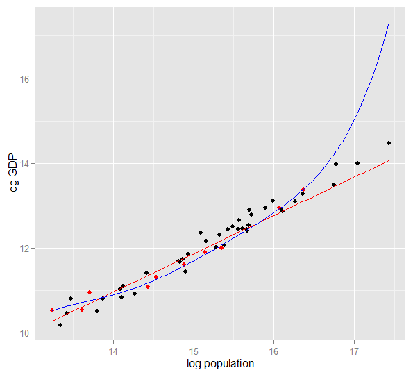
The coefficient estimates are much better for the correctly specified model. But note that the $R^2$ is lower, at 0.7961, as the less complex model has less flexibility in fitting the observed responses. $R^2$ is more dangerous than useful in this case!

fixed typos
Source Link
Scortchi
  • 31.6k
  • 9
  • 102
  • 281

Here is a plot of log GDP against log population for 50 US states in 2010. A random sample of 10 states was selected (hightlightedhighlighted in red) and for that sample we fit a simple linear model and a polynomial of degree 5. For the sample points, the polynomial has extra degrees of freedom that let it "wriggle" closer to the observed data than the straight line can. But the 50 states as a whole obey a nearly linear relationship, so the predictive performance of the polynomial model on the 40 out-of-sample points is very poor compared to the less complex model, particularly when extrapolating. The polynomial was effectively fitting some of the random structure (noise) of the sample, which did not generalise to the wider population. It was particularly poor at extrapolating beyond the observed range of the sample. (Code plus data for this plot is at the bottom of this revision of this answer.)

  • Run the simulation several times and see how the results differ. You will find more variability using small sample sizes than large ones.
  • Try changing the sample sizes. If increased to, say, n <- 1e6, then the overfitted model eventually estimates reasonable coefficients (about 5 for intercept, about 2 for $x_1$, about 0 for everything else) and its predictive performance as measured by SSE doesn't trail the correctly specified model so badly. Conversely, try fitted basedfitting on a very small sample (bear in mind you need to leave enough degrees of freedom to estimate all the coefficients) and you will see that the overfitted model has appalling performance both for estimating coefficients and predicting for new data.
  • Try reducing the correlation between the predictor variables by playing with the off-diagonal elements of the variance-covariance matrix Sigma. Just remember to keep it positive semi-definite (which includes being symmetric). You should find if you reduce the multicollinearity, the overfitted model doesn't perform quite so badly. But bear in mind that correlated predictors do occur in real life.
  • Try experimenting with the specification of the overfitted model. What if you include polynomial terms?
  • What if you simulate data for a different region of predictors, rather than having their mean all around 5? If the correct data generating process for $y$ is still df$y <- 5 + 2*df$x1 + rnorm(n=nrow(df)), see how well the models fitted to the original data can predict that $y$. Depending on how you generate the $x_i$ values, you may find that extrapolation with the overfitted model produces predictions far worse than the correctly specified model.
  • What if you change the data generating process so that $y$ now depends, weakly, on $x_2$, $x3$ and perhaps the interactions as well? This may be a more realistic scenario that depending on $x_1$ alone. If you use e.g. df$y <- 5 + 2 * df$x1 + 0.1*df$x2 + 0.1*df$x3 + rnorm(n=nrow(df)) then $x_2$ and $x_3$ are "almost irrelevant", but not quite. (Note that I drew all the $x$ variables from the same range, so it does make sense to compare their coefficients like that.) Then the simple model involving only $x_1$ suffers omitted variable bias, though since $x_2$ and $x_3$ are not particularly important, this is not too severe. On a small sample, e.g. nsample <- 25, the full model is still overfitted, despite being a better representation of the underlying population, and on repeated simulations its predictive performance on the holdout set is still consistently worse. With such limited data, it's more important to get a good estimate for the coefficient of $x_1$ than to expend information on the luxury of estimating the less important coefficients. With the effects of $x_2$ and $x_3$ being so hard to discern in a small sample, the full model is effectively using the flexibility from its extra degrees of freedom to "fit the noise" and this generalises poorly. But with nsample <- 1e6, it can estimate the weaker effects pretty well, and simulations show the complex model has predictive power that outperforms the simple one. This shows how "overfitting" is an issue of both model complexity and the available data.

Here is a plot of log GDP against log population for 50 US states in 2010. A random sample of 10 states was selected (hightlighted in red) and for that sample we fit a simple linear model and a polynomial of degree 5. For the sample points, the polynomial has extra degrees of freedom that let it "wriggle" closer to the observed data than the straight line can. But the 50 states as a whole obey a nearly linear relationship, so the predictive performance of the polynomial model on the 40 out-of-sample points is very poor compared to the less complex model, particularly when extrapolating. The polynomial was effectively fitting some of the random structure (noise) of the sample, which did not generalise to the wider population. It was particularly poor at extrapolating beyond the observed range of the sample. (Code plus data for this plot is at the bottom of this revision of this answer.)

  • Run the simulation several times and see how the results differ. You will find more variability using small sample sizes than large ones.
  • Try changing the sample sizes. If increased to, say, n <- 1e6, then the overfitted model eventually estimates reasonable coefficients (about 5 for intercept, about 2 for $x_1$, about 0 for everything else) and its predictive performance as measured by SSE doesn't trail the correctly specified model so badly. Conversely, try fitted based on a very small sample (bear in mind you need to leave enough degrees of freedom to estimate all the coefficients) and you will see that the overfitted model has appalling performance both for estimating coefficients and predicting for new data.
  • Try reducing the correlation between the predictor variables by playing with the off-diagonal elements of the variance-covariance matrix Sigma. Just remember to keep it positive semi-definite (which includes being symmetric). You should find if you reduce the multicollinearity, the overfitted model doesn't perform quite so badly. But bear in mind that correlated predictors do occur in real life.
  • Try experimenting with the specification of the overfitted model. What if you include polynomial terms?
  • What if you simulate data for a different region of predictors, rather than having their mean all around 5? If the correct data generating process for $y$ is still df$y <- 5 + 2*df$x1 + rnorm(n=nrow(df)), see how well the models fitted to the original data can predict that $y$. Depending on how you generate the $x_i$ values, you may find that extrapolation with the overfitted model produces predictions far worse than the correctly specified model.
  • What if you change the data generating process so that $y$ now depends, weakly, on $x_2$, $x3$ and perhaps the interactions as well? This may be a more realistic scenario that depending on $x_1$ alone. If you use e.g. df$y <- 5 + 2 * df$x1 + 0.1*df$x2 + 0.1*df$x3 + rnorm(n=nrow(df)) then $x_2$ and $x_3$ are "almost irrelevant", but not quite. (Note that I drew all the $x$ variables from the same range, so it does make sense to compare their coefficients like that.) Then the simple model involving only $x_1$ suffers omitted variable bias, though since $x_2$ and $x_3$ are not particularly important, this is not too severe. On a small sample, e.g. nsample <- 25, the full model is still overfitted, despite being a better representation of the underlying population, and on repeated simulations its predictive performance on the holdout set is still consistently worse. With such limited data, it's more important to get a good estimate for the coefficient of $x_1$ than to expend information on the luxury of estimating the less important coefficients. With the effects of $x_2$ and $x_3$ being so hard to discern in a small sample, the full model is effectively using the flexibility from its extra degrees of freedom to "fit the noise" and this generalises poorly. But with nsample <- 1e6, it can estimate the weaker effects pretty well, and simulations show the complex model has predictive power that outperforms the simple one. This shows how "overfitting" is an issue of both model complexity and the available data.

Here is a plot of log GDP against log population for 50 US states in 2010. A random sample of 10 states was selected (highlighted in red) and for that sample we fit a simple linear model and a polynomial of degree 5. For the sample points, the polynomial has extra degrees of freedom that let it "wriggle" closer to the observed data than the straight line can. But the 50 states as a whole obey a nearly linear relationship, so the predictive performance of the polynomial model on the 40 out-of-sample points is very poor compared to the less complex model, particularly when extrapolating. The polynomial was effectively fitting some of the random structure (noise) of the sample, which did not generalise to the wider population. It was particularly poor at extrapolating beyond the observed range of the sample. (Code plus data for this plot is at the bottom of this revision of this answer.)

  • Run the simulation several times and see how the results differ. You will find more variability using small sample sizes than large ones.
  • Try changing the sample sizes. If increased to, say, n <- 1e6, then the overfitted model eventually estimates reasonable coefficients (about 5 for intercept, about 2 for $x_1$, about 0 for everything else) and its predictive performance as measured by SSE doesn't trail the correctly specified model so badly. Conversely, try fitting on a very small sample (bear in mind you need to leave enough degrees of freedom to estimate all the coefficients) and you will see that the overfitted model has appalling performance both for estimating coefficients and predicting for new data.
  • Try reducing the correlation between the predictor variables by playing with the off-diagonal elements of the variance-covariance matrix Sigma. Just remember to keep it positive semi-definite (which includes being symmetric). You should find if you reduce the multicollinearity, the overfitted model doesn't perform quite so badly. But bear in mind that correlated predictors do occur in real life.
  • Try experimenting with the specification of the overfitted model. What if you include polynomial terms?
  • What if you simulate data for a different region of predictors, rather than having their mean all around 5? If the correct data generating process for $y$ is still df$y <- 5 + 2*df$x1 + rnorm(n=nrow(df)), see how well the models fitted to the original data can predict that $y$. Depending on how you generate the $x_i$ values, you may find that extrapolation with the overfitted model produces predictions far worse than the correctly specified model.
  • What if you change the data generating process so that $y$ now depends, weakly, on $x_2$, $x3$ and perhaps the interactions as well? This may be a more realistic scenario that depending on $x_1$ alone. If you use e.g. df$y <- 5 + 2 * df$x1 + 0.1*df$x2 + 0.1*df$x3 + rnorm(n=nrow(df)) then $x_2$ and $x_3$ are "almost irrelevant", but not quite. (Note that I drew all the $x$ variables from the same range, so it does make sense to compare their coefficients like that.) Then the simple model involving only $x_1$ suffers omitted variable bias, though since $x_2$ and $x_3$ are not particularly important, this is not too severe. On a small sample, e.g. nsample <- 25, the full model is still overfitted, despite being a better representation of the underlying population, and on repeated simulations its predictive performance on the holdout set is still consistently worse. With such limited data, it's more important to get a good estimate for the coefficient of $x_1$ than to expend information on the luxury of estimating the less important coefficients. With the effects of $x_2$ and $x_3$ being so hard to discern in a small sample, the full model is effectively using the flexibility from its extra degrees of freedom to "fit the noise" and this generalises poorly. But with nsample <- 1e6, it can estimate the weaker effects pretty well, and simulations show the complex model has predictive power that outperforms the simple one. This shows how "overfitting" is an issue of both model complexity and the available data.
Post Undeleted by Silverfish
remove full code and include link to past revision instead
Source Link
Silverfish
  • 23.9k
  • 28
  • 105
  • 206

The basicA common problem ofthat results in overfitting in real life is that in addition to terms for a correctly specified model, we may have have added something extraneous: irrelevant powers (or other transformations) of the correct terms, irrelevant variables, or irrelevant interactions.

  • irrelevant powers (or other transformations) of the correct terms,
  • irrelevant variables,
  • irrelevant interactions.

This happens in multiple regression if you add a variable that should not appear in the correctly specified model but do not want to drop it because you are afraid of inducing omitted variable bias. Of course, you have no way of knowing you have wrongly included it, since you can't see the whole population, only your sample, so can't know for sure what the correct specification is. (As @Scortchi points out in the comments, there may be no such thing as a the "correct" model specification - in that sense, the aim of modelling is finding a "good enough" specification; to avoid overfitting involves avoiding a model complexity greater than can be sustained from the available data.) If you want a real-world example of overfitting, this happens every time you throw all the potential predictors into a regression model, should any of them in fact have no relationship with the response once the effects of others are partialled out.

TheWith this type of overfitting, the good news is that inclusion of these irrelevant terms does not introduce bias of your estimators, and in very large samples the coefficients of the irrelevant terms should be close to zero. But there is also bad news: because the limited information from your sample is now being used to estimate more parameters, it can only do so with less precision - so the standard errors on the genuinely relevant terms increase. That also means they're likely to be further from the true values than estimates from a correctly specified regression, which in turn means that if given new values of your explanatory variables, the predictions from the overfitted model will tend to be less accurate than for the correctly specified model.

As an aside, "extrapolation" - where you make predictions for your response variable based on values of your explanatory variables which do not come from the region you sampled from -Here is always dangerous (particularly if you don't have underlying theoretical/physical groundsa plot of log GDP against log population for your model specification - why should your model be correct50 US states in this new region2010. A random sample of predictors?), but making extrapolated predictions with an overfitted model can be especially dangerous.10 states was selected (When I have time I will add some graphs to explain this, buthightlighted in red) and for now: imagine if the true relationship isthat sample we fit a simple linear butmodel and a 7th powerpolynomial of degree 5. For the sample points, the polynomial has been overfittedextra degrees of freedom that let it "wriggle" closer to the observed data than the straight line can. Extrapolation would beBut the 50 states as a terrible ideawhole obey a nearly linear relationship, so the predictive performance of the polynomial model on the 40 out-of-sample points is very poor compared to the less complex model, particularly when extrapolating. The polynomial was effectively fitting some of the random structure (noise) of the sample, which did not generalise to the wider population. It was particularly poor at extrapolating beyond the observed range of the sample. (Code plus data for this plot is at the bottom of this revision of this answer.)

Extrapolation from overly complex model

Similar issues affect regression against multiple predictors. To look at some actual data, it's easier with simulation rather than real-world samples since this way you control the data-generating process (effectively, you get to see the "population" and the true relationship). In this R code, the true model is $y_i = 2x_{1,i} + 5 + \epsilon_i$ but data is also provided on irrelevant variables $x_2$ and $x_3$. I have designed the simulation so that the the predictor variables are correlated, which would be a common occurrence in real-life data, particularly in the social sciences. We fit models which are correctly specified and overfitted (includes the irrelevant predictors and their interactions) on one portion of the generated data, then compare predictive performance on a holdout set. The multicollinearity of the predictors makes life even harder for the overfitted model, since it becomes harder for it to pick apart the effects of $x_1$, $x_2$ and $x_3$, but note that this does not bias any of the coefficient estimators.

require(MASS) #for multivariate normal simulation
     
nnsample <- 10025   #sample to regress plus holdout
holdoutnholdout <- 50 #removed from sample1e6 size to#to check model predictions
Sigma <- matrix(c(1, 0.5, 0.4, 0.5, 1, 0.3, 0.4, 0.3, 1), nrow=3)
df <- as.data.frame(mvrnorm(n=nn=(nsample+nholdout), mu=c(5,5,5), Sigma=Sigma))
colnames(df) <- c("x1", "x2", "x3")
df$y <- 5 + 2 * df$x1 + rnorm(n=nrow(df)) #y = 5 + *x1 + e

holdout.df <- df[1:holdoutnholdout,]
regress.df <- df[(holdout+1nholdout+1):n(nholdout+nsample),]

overfit.lm <- lm(y ~ x1*x2*x3, regress.df)
correctspec.lm <- lm(y ~ x1, regress.df)
summary(overfit.lm)
anova(overfit.lm)
summary(correctspec.lm)
anova(correctspec.lm)

holdout.df$overfitPred <- predict.lm(overfit.lm, newdata=holdout.df)
holdout.df$correctSpecPred <- predict.lm(correctspec.lm, newdata=holdout.df)
with(holdout.df, sum((y - overfitPred)^2)) #SSE
with(holdout.df, sum((y - correctSpecPred)^2))

require(ggplot2)
errors.df <- data.frame(
    Model = rep(c("Overfitted", "Correctly specified"), each=nholdout),
    Error = with(holdout.df, c(y - overfitPred, y - correctSpecPred)))
ggplot(errors.df, aes(x=Error, color=Model)) + geom_density(size=1) +
    theme(legend.position="bottom")

Here are my results from one run, but it's best to run the simulation several times to see the effect of different generated samples.

>     summary(overfit.lm)

Call:
lm(formula = y ~ x1 * x2 * x3, data = regress.df)

Residuals:
     Min       1Q   Median       3Q      Max 
-12.9297422294 -0.59009 63142 -0.0056609491  0.4541351983  2.3190124193 

Coefficients:
            Estimate Std. Error t value Pr(>|t|)
(Intercept)  1518.5925 85992   1165.259400775   10.385290    0.173775
x1           -02.1485  40912   211.739090433  -0.054202    0.957842
x2           -12.8888  13777   212.309548892  -0.818171    0.418866
x3           -31.7341  13941   212.714894670  -10.375088    0.176931
x1:x2         0.3699 78280    02.501425867   0.738347    0.465733
x1:x3         0.7816 53616    02.612730834   10.276232    0.209819
x2:x3         0.6643 08019    02.524149028   10.268032    0.212975
x1:x2:x3     -0.1355 08584    0.107343891  -10.262196    0.214847

Residual standard error: 1.037101 on 4217 degrees of freedom
Multiple R-squared: 0.83128297,     Adjusted R-squared: 0.8037596 
F-statistic: 2911.5484 on 7 and 4217 DF,  p-value: 21.862e942e-14 05

These coefficient estimates for the overfitted model are terrible - should be about 5 for the intercept, 2 for $x_1$ and 0 for the rest. But the standard errors are also large. The correct values for those parameters do lie well within the 95% confidence intervals in each case. But theThe $R^2$ is 0.83128297 which suggests a reasonable fit.

>     summary(correctspec.lm)

Call:
lm(formula = y ~ x1, data = regress.df)

Residuals:
    Min      1Q  Median      3Q     Max 
-12.85674951 -0.78094112 -0.10702000  0.46857876  2.68391706 

Coefficients:
            Estimate Std. Error t value Pr(>|t|)    
(Intercept)   4.97887844     01.68921272   74.224244 30.34e-09000306 ***
x1            21.00869974     0.1396 2108 14.391  <9.476 2e2.09e-1609 ***
---
Signif. codes:  0 ‘***’ 0.001 ‘**’ 0.01 ‘*’ 0.05 ‘.’ 0.1 ‘ ’ 1 

Residual standard error: 1.024036 on 4823 degrees of freedom
Multiple R-squared: 0.81187961,     Adjusted R-squared: 0.80797872 
F-statistic: 207 89.18 on 1 and 4823 DF,  p-value: < 2.2e089e-1609

The coefficient estimates are much better for the correctly specified model. But note that the $R^2$ is lower, at 0.81187961, as the less complex model has less flexibility in fitting the observed responses. So we can see $R^2$ beingis more dangerous than useful in this case!

>     with(holdout.df, sum((y - overfitPred)^2)) #SSE
[1] 89.666711271557
>     with(holdout.df, sum((y - correctSpecPred)^2))
[1] 60.799181052217

The higher $R^2$ on the sample we regressed on showed how the overfitted model produced predictions, $\hat{y}$, that were closer to the observed $y$ than the correctly specified model could. But that's because it was overfitting to that data (and had more degrees of freedom to do so than the correctly specified model did, so could produce a "better" fit). Look at the Sum of Squared Errors for the predictions on the holdout set, which we didn't use to estimate the regression coefficients from, and we can see how much worse the overfitted model has performed. In reality the correctly specified model is the one which makes the best predictions. We shouldn't base our assessment of the predictive performance on the results from the set of data we used to estimate the models. Here's a density plot of the errors, with the correct model specification producing more errors close to 0:
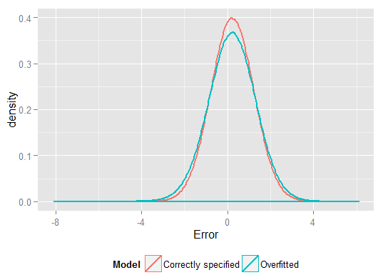
Prediction errors on holdout set

  • Run the simulation several times and see how the results differ. You will find more variability using small sample sizes than large ones.
  • Try changing the sample sizes. You should find that by the time you increaseIf increased to about, say, n <- 2e8 and holdout <- 1e81e6 that, then the overfitted model eventually estimates fairly reasonable coefficients (about 5 for intercept, about 2 for $x_1$, about 0 for everything else) and its predictive performance as measured by SSE doesn't trail the correctly specified model so badly. Conversely, try fitted based on a very small sample (bear in mind you need to leave enough degrees of freedom to estimate all the coefficients) and you will see that the overfitted model has appalling performance both for estimating coefficients and predicting for new data.
  • Try reducing the correlation between the predictor variables by playing with the off-diagonal elements of the variance-covariance matrix Sigma. Just remember to keep it positive semi-definite (which includes being symmetric). You should find if you reduce the multicollinearity, the overfitted model doesn't perform quite so badly. But bear in mind that correlated predictors do occur in real life.
  • Try experimenting with the specification of the overfitted model. What if you include polynomial terms?
  • What if you simulate data for a different region of predictors, rather than having their mean all around 5? If the correct data generating process for $y$ is still df$y <- 5 + 2 * df$x12*df$x1 + rnorm(n=nrow(df)), see how well the models fitted to the original data can predict that $y$. Depending on how you generate the $x_i$ values, you may find that extrapolation with the overfitted model produces predictions far worse than the correctly specified model.
  • What if you change the data generating process so that $y$ now depends, weakly, on $x_2$, $x3$ and perhaps the interactions as well? This may be a more realistic scenario that depending on $x_1$ alone. If you use e.g. df$y <- 5 + 2 * df$x1 + 0.1*df$x2 + 0.1*df$x3 + rnorm(n=nrow(df)) then $x_2$ and $x_3$ are "almost irrelevant", but not quite. (Note that I drew all the $x$ variables from the same range, so it does make sense to compare their coefficients like that.) Then the simple model involving only $x_1$ suffers omitted variable bias, though since $x_2$ and $x_3$ are not particularly important, this is not too severe. On a small sample, e.g. nsample <- 25, the full model is still overfitted, despite being a better representation of the underlying population, and on repeated simulations its predictive performance on the holdout set is still consistently worse. With such limited data, it's more important to get a good estimate for the coefficient of $x_1$ than to expend information on the luxury of estimating the less important coefficients. With the effects of $x_2$ and $x_3$ being so hard to discern in a small sample, the full model is effectively using the flexibility from its extra degrees of freedom to "fit the noise" and this generalises poorly. But with nsample <- 1e6, it can estimate the weaker effects pretty well, and simulations show the complex model has predictive power that outperforms the simple one. This shows how "overfitting" is an issue of both model complexity and the available data.

The basic problem of overfitting is that in addition to terms for a correctly specified model, we may have have added:

  • irrelevant powers (or other transformations) of the correct terms,
  • irrelevant variables,
  • irrelevant interactions.

This happens in multiple regression if you add a variable that should not appear in the correctly specified model but do not want to drop it because you are afraid of inducing omitted variable bias. Of course, you have no way of knowing you have wrongly included it, since you can't see the whole population, only your sample, so can't know for sure what the correct specification is. If you want a real-world example of overfitting, this happens every time you throw all the potential predictors into a regression model, should any of them in fact have no relationship with the response once the effects of others are partialled out.

The good news is that inclusion of these irrelevant terms does not introduce bias of your estimators, and in very large samples the coefficients of the irrelevant terms should be close to zero. But there is also bad news: because the limited information from your sample is now being used to estimate more parameters, it can only do so with less precision - so the standard errors on the genuinely relevant terms increase. That also means they're likely to be further from the true values than estimates from a correctly specified regression, which in turn means that if given new values of your explanatory variables, the predictions from the overfitted model will tend to be less accurate than for the correctly specified model.

As an aside, "extrapolation" - where you make predictions for your response variable based on values of your explanatory variables which do not come from the region you sampled from - is always dangerous (particularly if you don't have underlying theoretical/physical grounds for your model specification - why should your model be correct in this new region of predictors?), but making extrapolated predictions with an overfitted model can be especially dangerous. (When I have time I will add some graphs to explain this, but for now: imagine if the true relationship is linear but a 7th power polynomial has been overfitted to the data. Extrapolation would be a terrible idea.)

To look at some actual data, it's easier with simulation rather than real-world samples since this way you control the data-generating process (effectively, you get to see the "population" and the true relationship). In this R code, the true model is $y_i = 2x_{1,i} + 5 + \epsilon_i$ but data is also provided on irrelevant variables $x_2$ and $x_3$. I have designed the simulation so that the the predictor variables are correlated, which would be a common occurrence in real-life data, particularly in the social sciences. We fit models which are correctly specified and overfitted (includes the irrelevant predictors and their interactions) on one portion of the generated data, then compare predictive performance on a holdout set. The multicollinearity of the predictors makes life even harder for the overfitted model, since it becomes harder for it to pick apart the effects of $x_1$, $x_2$ and $x_3$, but note that this does not bias any of the coefficient estimators.

require(MASS) #for multivariate normal simulation
 
n <- 100 #sample to regress plus holdout
holdout <- 50 #removed from sample size to check model predictions
Sigma <- matrix(c(1, 0.5, 0.4, 0.5, 1, 0.3, 0.4, 0.3, 1), nrow=3)
df <- as.data.frame(mvrnorm(n=n, mu=c(5,5,5), Sigma=Sigma))
colnames(df) <- c("x1", "x2", "x3")
df$y <- 5 + 2 * df$x1 + rnorm(n=nrow(df)) #y = 5 + *x1 + e

holdout.df <- df[1:holdout,]
regress.df <- df[(holdout+1):n,]

overfit.lm <- lm(y ~ x1*x2*x3, regress.df)
correctspec.lm <- lm(y ~ x1, regress.df)
summary(overfit.lm)
anova(overfit.lm)
summary(correctspec.lm)
anova(correctspec.lm)

holdout.df$overfitPred <- predict.lm(overfit.lm, newdata=holdout.df)
holdout.df$correctSpecPred <- predict.lm(correctspec.lm, newdata=holdout.df)
with(holdout.df, sum((y - overfitPred)^2))
with(holdout.df, sum((y - correctSpecPred)^2))

Here are my results.

> summary(overfit.lm)

Call:
lm(formula = y ~ x1 * x2 * x3, data = regress.df)

Residuals:
     Min       1Q   Median       3Q      Max 
-1.92974 -0.59009  0.00566  0.45413  2.31901 

Coefficients:
            Estimate Std. Error t value Pr(>|t|)
(Intercept)  15.5925    11.2594   1.385    0.173
x1           -0.1485     2.7390  -0.054    0.957
x2           -1.8888     2.3095  -0.818    0.418
x3           -3.7341     2.7148  -1.375    0.176
x1:x2         0.3699     0.5014   0.738    0.465
x1:x3         0.7816     0.6127   1.276    0.209
x2:x3         0.6643     0.5241   1.268    0.212
x1:x2:x3     -0.1355     0.1073  -1.262    0.214

Residual standard error: 1.037 on 42 degrees of freedom
Multiple R-squared: 0.8312,     Adjusted R-squared: 0.803 
F-statistic: 29.54 on 7 and 42 DF,  p-value: 2.862e-14 

These coefficient estimates for the overfitted model are terrible - should be about 5 for the intercept, 2 for $x_1$ and 0 for the rest. But the standard errors are also large. The correct values for those parameters do lie well within the 95% confidence intervals in each case. But the $R^2$ is 0.8312.

> summary(correctspec.lm)

Call:
lm(formula = y ~ x1, data = regress.df)

Residuals:
    Min      1Q  Median      3Q     Max 
-1.8567 -0.7809 -0.1070  0.4685  2.6839 

Coefficients:
            Estimate Std. Error t value Pr(>|t|)    
(Intercept)   4.9788     0.6892   7.224 3.34e-09 ***
x1            2.0086     0.1396  14.391  < 2e-16 ***
---
Signif. codes:  0 ‘***’ 0.001 ‘**’ 0.01 ‘*’ 0.05 ‘.’ 0.1 ‘ ’ 1 

Residual standard error: 1.024 on 48 degrees of freedom
Multiple R-squared: 0.8118,     Adjusted R-squared: 0.8079 
F-statistic: 207.1 on 1 and 48 DF,  p-value: < 2.2e-16

The coefficient estimates are much better for the correctly specified model. But note that the $R^2$ is lower, at 0.8118. So we can see $R^2$ being more dangerous than useful in this case!

> with(holdout.df, sum((y - overfitPred)^2))
[1] 89.66671
> with(holdout.df, sum((y - correctSpecPred)^2))
[1] 60.79918

The higher $R^2$ on the sample we regressed on showed how the overfitted model produced predictions, $\hat{y}$, that were closer to the observed $y$ than the correctly specified model could. But that's because it was overfitting to that data (and had more degrees of freedom to do so than the correctly specified model did, so could produce a "better" fit). Look at the Sum of Squared Errors for the predictions on the holdout set, which we didn't use to estimate the regression coefficients from, and we can see how much worse the overfitted model has performed. In reality the correctly specified model is the one which makes the best predictions. We shouldn't base our assessment of the predictive performance on the results from the set of data we used to estimate the models.

  • Run the simulation several times and see how the results differ. You will find more variability using small sample sizes than large ones.
  • Try changing the sample sizes. You should find that by the time you increase to about n <- 2e8 and holdout <- 1e8 that the overfitted model eventually estimates fairly reasonable coefficients (about 5 for intercept, about 2 for $x_1$, about 0 for everything else) and its predictive performance as measured by SSE doesn't trail the correctly specified model so badly. Conversely, try fitted based on a very small sample (bear in mind you need to leave enough degrees of freedom to estimate all the coefficients) and you will see that the overfitted model has appalling performance both for estimating coefficients and predicting for new data.
  • Try reducing the correlation between the predictor variables by playing with the off-diagonal elements of the variance-covariance matrix Sigma. Just remember to keep it positive semi-definite (which includes being symmetric). You should find if you reduce the multicollinearity, the overfitted model doesn't perform quite so badly. But bear in mind that correlated predictors do occur in real life.
  • Try experimenting with the specification of the overfitted model. What if you include polynomial terms?
  • What if you simulate data for a different region of predictors, rather than having their mean all around 5? If the correct data generating process for $y$ is still df$y <- 5 + 2 * df$x1 + rnorm(n=nrow(df)), see how well the models fitted to the original data can predict that $y$. Depending on how you generate the $x_i$ values, you may find that extrapolation with the overfitted model produces predictions far worse than the correctly specified model.

A common problem that results in overfitting in real life is that in addition to terms for a correctly specified model, we may have have added something extraneous: irrelevant powers (or other transformations) of the correct terms, irrelevant variables, or irrelevant interactions.

This happens in multiple regression if you add a variable that should not appear in the correctly specified model but do not want to drop it because you are afraid of inducing omitted variable bias. Of course, you have no way of knowing you have wrongly included it, since you can't see the whole population, only your sample, so can't know for sure what the correct specification is. (As @Scortchi points out in the comments, there may be no such thing as a the "correct" model specification - in that sense, the aim of modelling is finding a "good enough" specification; to avoid overfitting involves avoiding a model complexity greater than can be sustained from the available data.) If you want a real-world example of overfitting, this happens every time you throw all the potential predictors into a regression model, should any of them in fact have no relationship with the response once the effects of others are partialled out.

With this type of overfitting, the good news is that inclusion of these irrelevant terms does not introduce bias of your estimators, and in very large samples the coefficients of the irrelevant terms should be close to zero. But there is also bad news: because the limited information from your sample is now being used to estimate more parameters, it can only do so with less precision - so the standard errors on the genuinely relevant terms increase. That also means they're likely to be further from the true values than estimates from a correctly specified regression, which in turn means that if given new values of your explanatory variables, the predictions from the overfitted model will tend to be less accurate than for the correctly specified model.

Here is a plot of log GDP against log population for 50 US states in 2010. A random sample of 10 states was selected (hightlighted in red) and for that sample we fit a simple linear model and a polynomial of degree 5. For the sample points, the polynomial has extra degrees of freedom that let it "wriggle" closer to the observed data than the straight line can. But the 50 states as a whole obey a nearly linear relationship, so the predictive performance of the polynomial model on the 40 out-of-sample points is very poor compared to the less complex model, particularly when extrapolating. The polynomial was effectively fitting some of the random structure (noise) of the sample, which did not generalise to the wider population. It was particularly poor at extrapolating beyond the observed range of the sample. (Code plus data for this plot is at the bottom of this revision of this answer.)

Extrapolation from overly complex model

Similar issues affect regression against multiple predictors. To look at some actual data, it's easier with simulation rather than real-world samples since this way you control the data-generating process (effectively, you get to see the "population" and the true relationship). In this R code, the true model is $y_i = 2x_{1,i} + 5 + \epsilon_i$ but data is also provided on irrelevant variables $x_2$ and $x_3$. I have designed the simulation so that the the predictor variables are correlated, which would be a common occurrence in real-life data. We fit models which are correctly specified and overfitted (includes the irrelevant predictors and their interactions) on one portion of the generated data, then compare predictive performance on a holdout set. The multicollinearity of the predictors makes life even harder for the overfitted model, since it becomes harder for it to pick apart the effects of $x_1$, $x_2$ and $x_3$, but note that this does not bias any of the coefficient estimators.

require(MASS) #for multivariate normal simulation    
nsample <- 25   #sample to regress 
nholdout <- 1e6  #to check model predictions
Sigma <- matrix(c(1, 0.5, 0.4, 0.5, 1, 0.3, 0.4, 0.3, 1), nrow=3)
df <- as.data.frame(mvrnorm(n=(nsample+nholdout), mu=c(5,5,5), Sigma=Sigma))
colnames(df) <- c("x1", "x2", "x3")
df$y <- 5 + 2 * df$x1 + rnorm(n=nrow(df)) #y = 5 + *x1 + e

holdout.df <- df[1:nholdout,]
regress.df <- df[(nholdout+1):(nholdout+nsample),]

overfit.lm <- lm(y ~ x1*x2*x3, regress.df)
correctspec.lm <- lm(y ~ x1, regress.df)
summary(overfit.lm)
summary(correctspec.lm)

holdout.df$overfitPred <- predict.lm(overfit.lm, newdata=holdout.df)
holdout.df$correctSpecPred <- predict.lm(correctspec.lm, newdata=holdout.df)
with(holdout.df, sum((y - overfitPred)^2)) #SSE
with(holdout.df, sum((y - correctSpecPred)^2))

require(ggplot2)
errors.df <- data.frame(
    Model = rep(c("Overfitted", "Correctly specified"), each=nholdout),
    Error = with(holdout.df, c(y - overfitPred, y - correctSpecPred)))
ggplot(errors.df, aes(x=Error, color=Model)) + geom_density(size=1) +
    theme(legend.position="bottom")

Here are my results from one run, but it's best to run the simulation several times to see the effect of different generated samples.

>     summary(overfit.lm)

Call:
lm(formula = y ~ x1 * x2 * x3, data = regress.df)

Residuals:
     Min       1Q   Median       3Q      Max 
-2.22294 -0.63142 -0.09491  0.51983  2.24193 

Coefficients:
            Estimate Std. Error t value Pr(>|t|)
(Intercept) 18.85992   65.00775   0.290    0.775
x1          -2.40912   11.90433  -0.202    0.842
x2          -2.13777   12.48892  -0.171    0.866
x3          -1.13941   12.94670  -0.088    0.931
x1:x2        0.78280    2.25867   0.347    0.733
x1:x3        0.53616    2.30834   0.232    0.819
x2:x3        0.08019    2.49028   0.032    0.975
x1:x2:x3    -0.08584    0.43891  -0.196    0.847

Residual standard error: 1.101 on 17 degrees of freedom
Multiple R-squared: 0.8297,     Adjusted R-squared: 0.7596 
F-statistic: 11.84 on 7 and 17 DF,  p-value: 1.942e-05

These coefficient estimates for the overfitted model are terrible - should be about 5 for the intercept, 2 for $x_1$ and 0 for the rest. But the standard errors are also large. The correct values for those parameters do lie well within the 95% confidence intervals in each case. The $R^2$ is 0.8297 which suggests a reasonable fit.

>     summary(correctspec.lm)

Call:
lm(formula = y ~ x1, data = regress.df)

Residuals:
    Min      1Q  Median      3Q     Max 
-2.4951 -0.4112 -0.2000  0.7876  2.1706 

Coefficients:
            Estimate Std. Error t value Pr(>|t|)    
(Intercept)   4.7844     1.1272   4.244 0.000306 ***
x1            1.9974     0.2108   9.476 2.09e-09 ***
---
Signif. codes:  0 ‘***’ 0.001 ‘**’ 0.01 ‘*’ 0.05 ‘.’ 0.1 ‘ ’ 1 

Residual standard error: 1.036 on 23 degrees of freedom
Multiple R-squared: 0.7961,     Adjusted R-squared: 0.7872 
F-statistic:  89.8 on 1 and 23 DF,  p-value: 2.089e-09

The coefficient estimates are much better for the correctly specified model. But note that the $R^2$ is lower, at 0.7961, as the less complex model has less flexibility in fitting the observed responses. $R^2$ is more dangerous than useful in this case!

>     with(holdout.df, sum((y - overfitPred)^2)) #SSE
[1] 1271557
>     with(holdout.df, sum((y - correctSpecPred)^2))
[1] 1052217

The higher $R^2$ on the sample we regressed on showed how the overfitted model produced predictions, $\hat{y}$, that were closer to the observed $y$ than the correctly specified model could. But that's because it was overfitting to that data (and had more degrees of freedom to do so than the correctly specified model did, so could produce a "better" fit). Look at the Sum of Squared Errors for the predictions on the holdout set, which we didn't use to estimate the regression coefficients from, and we can see how much worse the overfitted model has performed. In reality the correctly specified model is the one which makes the best predictions. We shouldn't base our assessment of the predictive performance on the results from the set of data we used to estimate the models. Here's a density plot of the errors, with the correct model specification producing more errors close to 0:

Prediction errors on holdout set

  • Run the simulation several times and see how the results differ. You will find more variability using small sample sizes than large ones.
  • Try changing the sample sizes. If increased to, say, n <- 1e6, then the overfitted model eventually estimates reasonable coefficients (about 5 for intercept, about 2 for $x_1$, about 0 for everything else) and its predictive performance as measured by SSE doesn't trail the correctly specified model so badly. Conversely, try fitted based on a very small sample (bear in mind you need to leave enough degrees of freedom to estimate all the coefficients) and you will see that the overfitted model has appalling performance both for estimating coefficients and predicting for new data.
  • Try reducing the correlation between the predictor variables by playing with the off-diagonal elements of the variance-covariance matrix Sigma. Just remember to keep it positive semi-definite (which includes being symmetric). You should find if you reduce the multicollinearity, the overfitted model doesn't perform quite so badly. But bear in mind that correlated predictors do occur in real life.
  • Try experimenting with the specification of the overfitted model. What if you include polynomial terms?
  • What if you simulate data for a different region of predictors, rather than having their mean all around 5? If the correct data generating process for $y$ is still df$y <- 5 + 2*df$x1 + rnorm(n=nrow(df)), see how well the models fitted to the original data can predict that $y$. Depending on how you generate the $x_i$ values, you may find that extrapolation with the overfitted model produces predictions far worse than the correctly specified model.
  • What if you change the data generating process so that $y$ now depends, weakly, on $x_2$, $x3$ and perhaps the interactions as well? This may be a more realistic scenario that depending on $x_1$ alone. If you use e.g. df$y <- 5 + 2 * df$x1 + 0.1*df$x2 + 0.1*df$x3 + rnorm(n=nrow(df)) then $x_2$ and $x_3$ are "almost irrelevant", but not quite. (Note that I drew all the $x$ variables from the same range, so it does make sense to compare their coefficients like that.) Then the simple model involving only $x_1$ suffers omitted variable bias, though since $x_2$ and $x_3$ are not particularly important, this is not too severe. On a small sample, e.g. nsample <- 25, the full model is still overfitted, despite being a better representation of the underlying population, and on repeated simulations its predictive performance on the holdout set is still consistently worse. With such limited data, it's more important to get a good estimate for the coefficient of $x_1$ than to expend information on the luxury of estimating the less important coefficients. With the effects of $x_2$ and $x_3$ being so hard to discern in a small sample, the full model is effectively using the flexibility from its extra degrees of freedom to "fit the noise" and this generalises poorly. But with nsample <- 1e6, it can estimate the weaker effects pretty well, and simulations show the complex model has predictive power that outperforms the simple one. This shows how "overfitting" is an issue of both model complexity and the available data.
Post Deleted by Silverfish
added 651 characters in body
Source Link
Silverfish
  • 23.9k
  • 28
  • 105
  • 206
Loading
extent to which this is "real life"
Source Link
Silverfish
  • 23.9k
  • 28
  • 105
  • 206
Loading
Source Link
Silverfish
  • 23.9k
  • 28
  • 105
  • 206
Loading
Post Made Community Wiki by Silverfish