added 107 characters in body
Source Link
DWin
  • 7.8k
  • 23
  • 35

When you censor by simply choosing to randomly change the censoring variable, you are essentially leaving in all of the case-"times" under observation until just before they would have died during a complete observation model. (That is an egregious violation of the non-informative censoring assumption needed for survival analysis.) You need to change this to a model where the censoring process shortens time to a sensible (random) number for the censored cases.

censRand <- function(time, cens.t.5){  # cens.t.5 is the t 1/2 of censor process
  ctime <- rexp(n = length(time), rate = 1/cens.t.5)
  event <- (time <= ctime)
  t_obs <- pmin(time, ctime)
  return(data.frame(Times=t_obs, event=event))
}

time=rexp(1000, 4)
ctime <- censRand( time, 0.7)
plot( muhaz( ctime[ ,1], ctime[,2]) )
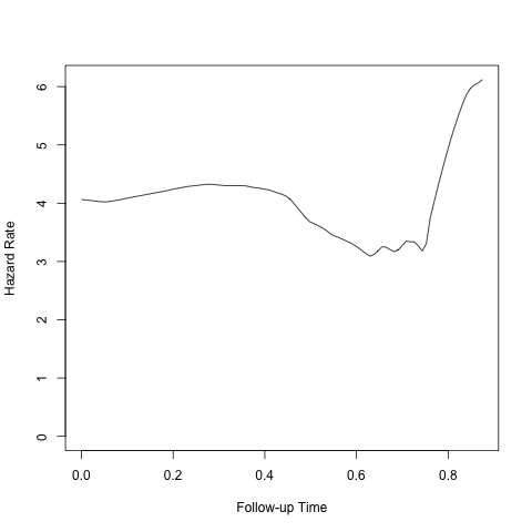
enter image description here

To get a further notion of the range of time over which this might be a "stable" estimate (if it were not already apparent from the excursions around the simulated parameter) you can run it multiple times:

png()
 plot( muhaz( ctime[ ,1], ctime[,2]) );
 for (i in 1:20) { time=rexp(1000, 4)
                    ctime <- censRand( time, 0.7)
                    lines( muhaz( ctime[ ,1], ctime[,2]) ) };
dev.off()
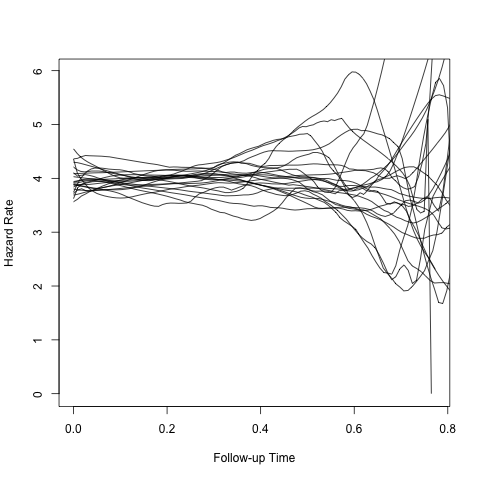
enter image description here

When you censor by simply choosing to randomly change the censoring variable, you are essentially leaving in all of the case-"times" under observation until just before they would have died during a complete observation model. You need to change this to a model where the censoring process shortens time to a sensible (random) number for the censored cases.

censRand <- function(time, cens.t.5){  # cens.t.5 is the t 1/2 of censor process
  ctime <- rexp(n = length(time), rate = 1/cens.t.5)
  event <- (time <= ctime)
  t_obs <- pmin(time, ctime)
  return(data.frame(Times=t_obs, event=event))
}

time=rexp(1000, 4)
ctime <- censRand( time, 0.7)
plot( muhaz( ctime[ ,1], ctime[,2]) )

enter image description here

To get a further notion of the range of time over which this might be a "stable" estimate (if it were not already apparent from the excursions around the simulated parameter) you can run it multiple times:

png()
 plot( muhaz( ctime[ ,1], ctime[,2]) );
 for (i in 1:20) { time=rexp(1000, 4)
                    ctime <- censRand( time, 0.7)
                    lines( muhaz( ctime[ ,1], ctime[,2]) ) };
dev.off()

enter image description here

When you censor by simply choosing to randomly change the censoring variable, you are essentially leaving in all of the case-"times" under observation until just before they would have died during a complete observation model. (That is an egregious violation of the non-informative censoring assumption needed for survival analysis.) You need to change this to a model where the censoring process shortens time to a sensible (random) number for the censored cases.

censRand <- function(time, cens.t.5){  # cens.t.5 is the t 1/2 of censor process
  ctime <- rexp(n = length(time), rate = 1/cens.t.5)
  event <- (time <= ctime)
  t_obs <- pmin(time, ctime)
  return(data.frame(Times=t_obs, event=event))
}

time=rexp(1000, 4)
ctime <- censRand( time, 0.7)
plot( muhaz( ctime[ ,1], ctime[,2]) )

enter image description here

To get a further notion of the range of time over which this might be a "stable" estimate (if it were not already apparent from the excursions around the simulated parameter) you can run it multiple times:

png()
 plot( muhaz( ctime[ ,1], ctime[,2]) );
 for (i in 1:20) { time=rexp(1000, 4)
                    ctime <- censRand( time, 0.7)
                    lines( muhaz( ctime[ ,1], ctime[,2]) ) };
dev.off()

enter image description here

added 526 characters in body
Source Link
DWin
  • 7.8k
  • 23
  • 35

When you censor by simply choosing to randomly change the censoring variable, you are essentially leaving in all of the case-"times" under observation until just before they would have died during a complete observation model. You need to change this to a model where the censoring process shortens time to a sensible (random) number for the censored cases.

censRand <- function(time, cens.t.5){  # cens.t.5 is the t 1/2 of censor process
  ctime <- rexp(n = length(time), rate = 1/cens.t.5)
  event <- (time <= ctime)
  t_obs <- pmin(time, ctime)
  return(data.frame(Times=t_obs, event=event))
}

time=rexp(1000, 4)
ctime <- censRand( time, 0.7)
plot( muhaz( ctime[ ,1], ctime[,2]) )

enter image description here

To get a further notion of the range of time over which this might be a "stable" estimate (if it were not already apparent from the excursions around the simulated parameter) you can run it multiple times:

png()
 plot( muhaz( ctime[ ,1], ctime[,2]) );
 for (i in 1:20) { time=rexp(1000, 4)
                    ctime <- censRand( time, 0.7)
                    lines( muhaz( ctime[ ,1], ctime[,2]) ) };
dev.off()

enter image description here

When you censor by simply choosing to randomly change the censoring variable, you are essentially leaving in all of the case-"times" under observation until just before they would have died during a complete observation model. You need to change this to a model where the censoring process shortens time to a sensible (random) number for the censored cases.

censRand <- function(time, cens.t.5){  # cens.t.5 is the t 1/2 of censor process
  ctime <- rexp(n = length(time), rate = 1/cens.t.5)
  event <- (time <= ctime)
  t_obs <- pmin(time, ctime)
  return(data.frame(Times=t_obs, event=event))
}

time=rexp(1000, 4)
ctime <- censRand( time, 0.7)
plot( muhaz( ctime[ ,1], ctime[,2]) )

enter image description here

To get a further notion of the range of time over which this might be a "stable" estimate (if it were not already apparent from the excursions around the simulated parameter) you can run it multiple times:

png()
 plot( muhaz( ctime[ ,1], ctime[,2]) );
 for (i in 1:20) { time=rexp(1000, 4)
                    ctime <- censRand( time, 0.7)
                    lines( muhaz( ctime[ ,1], ctime[,2]) ) };
dev.off()

enter image description here

Source Link
DWin
  • 7.8k
  • 23
  • 35

When you censor by simply choosing to randomly change the censoring variable, you are essentially leaving in all of the case-"times" under observation until just before they would have died during a complete observation model. You need to change this to a model where the censoring process shortens time to a sensible (random) number for the censored cases.

censRand <- function(time, cens.t.5){  # cens.t.5 is the t 1/2 of censor process
  ctime <- rexp(n = length(time), rate = 1/cens.t.5)
  event <- (time <= ctime)
  t_obs <- pmin(time, ctime)
  return(data.frame(Times=t_obs, event=event))
}

time=rexp(1000, 4)
ctime <- censRand( time, 0.7)
plot( muhaz( ctime[ ,1], ctime[,2]) )

enter image description here