edited tags
Link
kjetil b halvorsen
  • 82.8k
  • 32
  • 201
  • 663
Tweeted twitter.com/StackStats/status/655338033328300032
edited body
Source Link
lum
  • 354
  • 1
  • 12

Suppose I have two Beta random variables $$ X \sim \text{Beta}(a, b), \\ Y \sim \text{Beta}(ca, cb), $$ with $c > 1$. They both have same mean $\tfrac{a}{a+b}$, but $Y$ is more "peaky" than $X$. My question is as follows. Let $t \ge 0$; does $$ \mathbb{E}(e^{-tX}) \ge \mathbb{E}(e^{-kY}) \;\; \text{?} $$$$ \mathbb{E}(e^{-tX}) \ge \mathbb{E}(e^{-tY}) \;\; \text{?} $$ My intuition says yes, because $X$ "spreads" the weight more, therefore taps into the places where $e^{-kx}$$e^{-tx}$ is large. The case $t = 0$ is trivial, but I would like to prove it for $t > 0$.

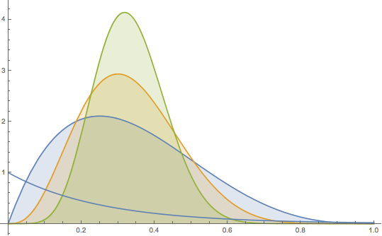
Here is a mathematica plot, with $t = 4$, and $(a, b) \in \{(2,4), (4,8), (8,16)\}$.

p1 = Plot[
   Evaluate@
    Table[PDF[BetaDistribution[\[Alpha], 2*\[Alpha]], 
      x], {\[Alpha], {2, 4, 8}}], {x, 0, 1}, Filling -> Axis];
p2 = Plot[Exp[-4 x], {x, 0, 1}];
Show[p1, p2]

beta pdfs and exponential fct

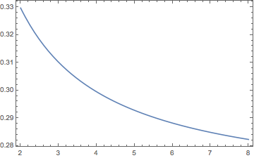
and the expectations, providing some empirical support to my claim:

Plot[Hypergeometric1F1[x, 3 x, -4], {x, 2, 8}, Frame -> True]

enter image description here

Note: I know that the expectation I'm trying to compute is just the moment generating function of the Beta distribution evaluated at negative values. This MGF is Kummer's confluent hypergeometric function of the first kind: $\mathbb{E}(e^{-tX}) = {}_1F_1(a, a+b, -t)$. I've spent quite a bit of time investigating this function, and nothing came out of it.

Suppose I have two Beta random variables $$ X \sim \text{Beta}(a, b), \\ Y \sim \text{Beta}(ca, cb), $$ with $c > 1$. They both have same mean $\tfrac{a}{a+b}$, but $Y$ is more "peaky" than $X$. My question is as follows. Let $t \ge 0$; does $$ \mathbb{E}(e^{-tX}) \ge \mathbb{E}(e^{-kY}) \;\; \text{?} $$ My intuition says yes, because $X$ "spreads" the weight more, therefore taps into the places where $e^{-kx}$ is large. The case $t = 0$ is trivial, but I would like to prove it for $t > 0$.

Here is a mathematica plot, with $t = 4$, and $(a, b) \in \{(2,4), (4,8), (8,16)\}$.

p1 = Plot[
   Evaluate@
    Table[PDF[BetaDistribution[\[Alpha], 2*\[Alpha]], 
      x], {\[Alpha], {2, 4, 8}}], {x, 0, 1}, Filling -> Axis];
p2 = Plot[Exp[-4 x], {x, 0, 1}];
Show[p1, p2]

beta pdfs and exponential fct

and the expectations, providing some empirical support to my claim:

Plot[Hypergeometric1F1[x, 3 x, -4], {x, 2, 8}, Frame -> True]

enter image description here

Note: I know that the expectation I'm trying to compute is just the moment generating function of the Beta distribution evaluated at negative values. This MGF is Kummer's confluent hypergeometric function of the first kind: $\mathbb{E}(e^{-tX}) = {}_1F_1(a, a+b, -t)$. I've spent quite a bit of time investigating this function, and nothing came out of it.
Suppose I have two Beta random variables $$ X \sim \text{Beta}(a, b), \\ Y \sim \text{Beta}(ca, cb), $$ with $c > 1$. They both have same mean $\tfrac{a}{a+b}$, but $Y$ is more "peaky" than $X$. My question is as follows. Let $t \ge 0$; does $$ \mathbb{E}(e^{-tX}) \ge \mathbb{E}(e^{-tY}) \;\; \text{?} $$ My intuition says yes, because $X$ "spreads" the weight more, therefore taps into the places where $e^{-tx}$ is large. The case $t = 0$ is trivial, but I would like to prove it for $t > 0$.

Here is a mathematica plot, with $t = 4$, and $(a, b) \in \{(2,4), (4,8), (8,16)\}$.

p1 = Plot[
   Evaluate@
    Table[PDF[BetaDistribution[\[Alpha], 2*\[Alpha]], 
      x], {\[Alpha], {2, 4, 8}}], {x, 0, 1}, Filling -> Axis];
p2 = Plot[Exp[-4 x], {x, 0, 1}];
Show[p1, p2]

beta pdfs and exponential fct

and the expectations, providing some empirical support to my claim:

Plot[Hypergeometric1F1[x, 3 x, -4], {x, 2, 8}, Frame -> True]

enter image description here

Note: I know that the expectation I'm trying to compute is just the moment generating function of the Beta distribution evaluated at negative values. This MGF is Kummer's confluent hypergeometric function of the first kind: $\mathbb{E}(e^{-tX}) = {}_1F_1(a, a+b, -t)$. I've spent quite a bit of time investigating this function, and nothing came out of it.

Source Link
lum
  • 354
  • 1
  • 12

Expectation of convex function of a Beta random variable

Suppose I have two Beta random variables $$ X \sim \text{Beta}(a, b), \\ Y \sim \text{Beta}(ca, cb), $$ with $c > 1$. They both have same mean $\tfrac{a}{a+b}$, but $Y$ is more "peaky" than $X$. My question is as follows. Let $t \ge 0$; does $$ \mathbb{E}(e^{-tX}) \ge \mathbb{E}(e^{-kY}) \;\; \text{?} $$ My intuition says yes, because $X$ "spreads" the weight more, therefore taps into the places where $e^{-kx}$ is large. The case $t = 0$ is trivial, but I would like to prove it for $t > 0$.

Here is a mathematica plot, with $t = 4$, and $(a, b) \in \{(2,4), (4,8), (8,16)\}$.

p1 = Plot[
   Evaluate@
    Table[PDF[BetaDistribution[\[Alpha], 2*\[Alpha]], 
      x], {\[Alpha], {2, 4, 8}}], {x, 0, 1}, Filling -> Axis];
p2 = Plot[Exp[-4 x], {x, 0, 1}];
Show[p1, p2]

beta pdfs and exponential fct

and the expectations, providing some empirical support to my claim:

Plot[Hypergeometric1F1[x, 3 x, -4], {x, 2, 8}, Frame -> True]

enter image description here

Note: I know that the expectation I'm trying to compute is just the moment generating function of the Beta distribution evaluated at negative values. This MGF is Kummer's confluent hypergeometric function of the first kind: $\mathbb{E}(e^{-tX}) = {}_1F_1(a, a+b, -t)$. I've spent quite a bit of time investigating this function, and nothing came out of it.