added 112 characters in body
Source Link
kjetil b halvorsen
  • 82.8k
  • 32
  • 201
  • 663

For those wanting to use a ggplot2 approach in R consider the facetshade function in the package extracat. This offers a general approach, not just for line plots. Here is an example with scatterplots (from the foot of this page):

data(olives, package="extracat")
library(scales)
fs1 <- facetshade(data = olives,
                  aes(x = palmitic, y = palmitoleic), f = 
                      .~Area ~ Area)
fs1 + geom_point(colour = alpha("black", 0.05)) +
      geom_point(data = olives, colour = "red") +
      facet_wrap(f=~Area, nrow=3) + 
          theme(legend.position="none")

enter image description here


EDIT: Using Adrian's simulated dataset from his earlier answer:

library(extracat)
facetshade(df, aes(x=time, y=y), f = .~label, bg.all = FALSE, 
            keep.orig = TRUE) +
           geom_line(aes(x=time, y=y, 
             group=orig.label),colour = alpha(1,0.3)) +
           geom_line(data=df, aes(colour=label), size = 1.2) 
           + xlab("") + ylab("")

Another approach is to draw two separate layers, one for the background and one for the highlighted cases. The trick is to draw the background layer using the dataset without the faceting variable. For the olive oil dataset the code is:

data(olives, package="extracat")
ggplot(olives, aes(palmitic, palmitoleic)) + 
  facet_wrap(~Area, nrow=3) + 
  geom_point(data=olives %>% select(-Area), 
        colour=alpha("black", 0.05)) + 
  geom_point(data=olives, colour="red") + 
  theme(legend.position="none")

For those wanting to use a ggplot2 approach in R consider the facetshade function in the package extracat. This offers a general approach, not just for line plots. Here is an example with scatterplots (from the foot of this page):

data(olives, package="extracat")
library(scales)
fs1 <- facetshade(data = olives,
                  aes(x = palmitic, y = palmitoleic), f = .~Area)
fs1 + geom_point(colour = alpha("black", 0.05)) +
      geom_point(data = olives, colour = "red") +
      facet_wrap(f=~Area, nrow=3) + theme(legend.position="none")

enter image description here


EDIT: Using Adrian's simulated dataset from his earlier answer:

library(extracat)
facetshade(df, aes(x=time, y=y), f = .~label, bg.all = FALSE, keep.orig = TRUE) +
           geom_line(aes(x=time, y=y, group=orig.label),colour = alpha(1,0.3)) +
           geom_line(data=df, aes(colour=label), size = 1.2) + xlab("") + ylab("")

Another approach is to draw two separate layers, one for the background and one for the highlighted cases. The trick is to draw the background layer using the dataset without the faceting variable. For the olive oil dataset the code is:

data(olives, package="extracat")
ggplot(olives, aes(palmitic, palmitoleic)) + 
  facet_wrap(~Area, nrow=3) + 
  geom_point(data=olives %>% select(-Area), colour=alpha("black", 0.05)) + 
  geom_point(data=olives, colour="red") + 
  theme(legend.position="none")
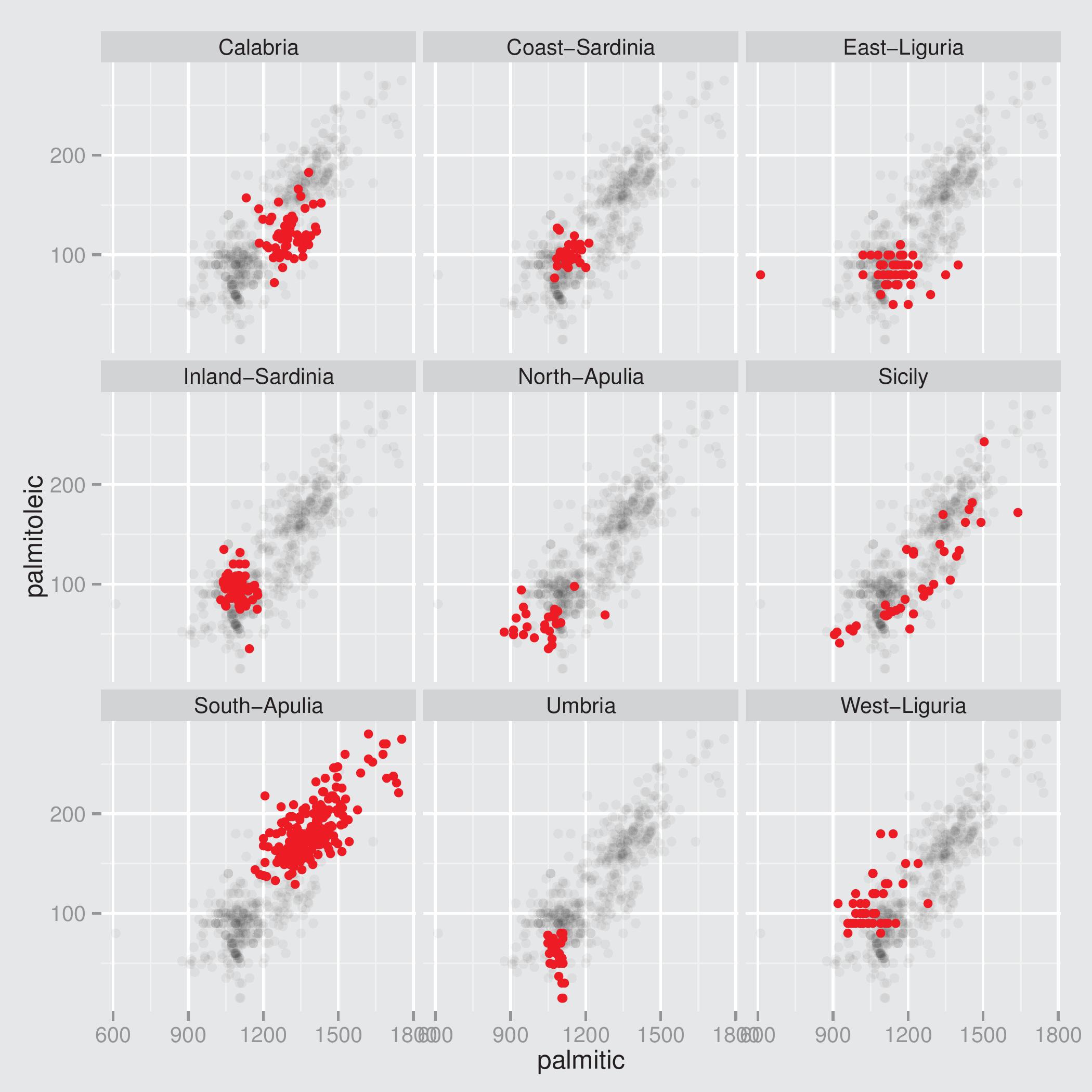
For those wanting to use a ggplot2 approach in R consider the facetshade function in the package extracat. This offers a general approach, not just for line plots. Here is an example with scatterplots (from the foot of this page):

data(olives, package="extracat")
library(scales)
fs1 <- facetshade(data = olives,
                  aes(x = palmitic, y = palmitoleic), f = 
                      . ~ Area)
fs1 + geom_point(colour = alpha("black", 0.05)) +
      geom_point(data = olives, colour = "red") +
      facet_wrap(f=~Area, nrow=3) + 
          theme(legend.position="none")

enter image description here


EDIT: Using Adrian's simulated dataset from his earlier answer:

library(extracat)
facetshade(df, aes(x=time, y=y), f = .~label, bg.all = FALSE, 
            keep.orig = TRUE) +
           geom_line(aes(x=time, y=y, 
             group=orig.label),colour = alpha(1,0.3)) +
           geom_line(data=df, aes(colour=label), size = 1.2) 
           + xlab("") + ylab("")

Another approach is to draw two separate layers, one for the background and one for the highlighted cases. The trick is to draw the background layer using the dataset without the faceting variable. For the olive oil dataset the code is:

data(olives, package="extracat")
ggplot(olives, aes(palmitic, palmitoleic)) + 
  facet_wrap(~Area, nrow=3) + 
  geom_point(data=olives %>% select(-Area), 
        colour=alpha("black", 0.05)) + 
  geom_point(data=olives, colour="red") + 
  theme(legend.position="none")
fit code in window; removed extra comment
Source Link
gung - Reinstate Monica
  • 147.5k
  • 89
  • 406
  • 716

For those wanting to use a ggplot2 approach in R consider the facetshade function in the package extracat. This offers a general approach, not just for line plots. Here is an example with scatterplots (from the foot of this page):

data(olives, package="extracat")
library(scales)
fs1 <- facetshade(data = olives,
                  aes(x = palmitic, y = palmitoleic), f = .~Area)
fs1 + geom_point(colour = alpha("black", 0.05)) +
      geom_point(data = olives, colour = "red") +
      facet_wrap(f=~Area, nrow=3) + theme(legend.position="none")

enter image description here


EDIT: Using Adrian's simulated dataset from his earlier answer:

library(extracat)
facetshade(df, aes(x=time, y=y), f = .~label, bg.all = FALSE, keep.orig = TRUE) +
           geom_line(aes(x=time, y=y, group=orig.label),colour = alpha(1,0.3)) +
           geom_line(data=df, aes(colour=label), size = 1.2) + xlab("") + ylab("")

Thanks for the editing. AnotherAnother approach is to draw two separate layers, one for the background and one for the highlighted cases. The trick is to draw the background layer using the dataset without the faceting variable. For the olive oil dataset the code is:

data(olives, package="extracat")
ggplot(olives, aes(palmitic, palmitoleic)) + 
  facet_wrap(~Area, nrow=3) + 
  geom_point(data=olives %>% select(-Area), colour = alphacolour=alpha("black", 0.05)) + geom_point(data 
 = olivesgeom_point(data=olives, colour = "red"colour="red") + 
  theme(legend.position="none")

For those wanting to use a ggplot2 approach in R consider the facetshade function in the package extracat. This offers a general approach, not just for line plots. Here is an example with scatterplots (from the foot of this page):

data(olives, package="extracat")
library(scales)
fs1 <- facetshade(data = olives,
                  aes(x = palmitic, y = palmitoleic), f = .~Area)
fs1 + geom_point(colour = alpha("black", 0.05)) +
      geom_point(data = olives, colour = "red") +
      facet_wrap(f=~Area, nrow=3) + theme(legend.position="none")

enter image description here


EDIT: Using Adrian's simulated dataset from his earlier answer:

library(extracat)
facetshade(df, aes(x=time, y=y), f = .~label, bg.all = FALSE, keep.orig = TRUE) +
           geom_line(aes(x=time, y=y, group=orig.label),colour = alpha(1,0.3)) +
           geom_line(data=df, aes(colour=label), size = 1.2) + xlab("") + ylab("")

Thanks for the editing. Another approach is to draw two separate layers, one for the background and one for the highlighted cases. The trick is to draw the background layer using the dataset without the faceting variable. For the olive oil dataset the code is:

data(olives, package="extracat")
ggplot(olives, aes(palmitic, palmitoleic)) + facet_wrap(~Area, nrow=3) + geom_point(data=olives %>% select(-Area), colour = alpha("black", 0.05)) + geom_point(data = olives, colour = "red") + theme(legend.position="none")

For those wanting to use a ggplot2 approach in R consider the facetshade function in the package extracat. This offers a general approach, not just for line plots. Here is an example with scatterplots (from the foot of this page):

data(olives, package="extracat")
library(scales)
fs1 <- facetshade(data = olives,
                  aes(x = palmitic, y = palmitoleic), f = .~Area)
fs1 + geom_point(colour = alpha("black", 0.05)) +
      geom_point(data = olives, colour = "red") +
      facet_wrap(f=~Area, nrow=3) + theme(legend.position="none")

enter image description here


EDIT: Using Adrian's simulated dataset from his earlier answer:

library(extracat)
facetshade(df, aes(x=time, y=y), f = .~label, bg.all = FALSE, keep.orig = TRUE) +
           geom_line(aes(x=time, y=y, group=orig.label),colour = alpha(1,0.3)) +
           geom_line(data=df, aes(colour=label), size = 1.2) + xlab("") + ylab("")

Another approach is to draw two separate layers, one for the background and one for the highlighted cases. The trick is to draw the background layer using the dataset without the faceting variable. For the olive oil dataset the code is:

data(olives, package="extracat")
ggplot(olives, aes(palmitic, palmitoleic)) + 
  facet_wrap(~Area, nrow=3) + 
  geom_point(data=olives %>% select(-Area), colour=alpha("black", 0.05)) +  
  geom_point(data=olives, colour="red") + 
  theme(legend.position="none")
Added alternative approach
Source Link

For those wanting to use a ggplot2 approach in R consider the facetshade function in the package extracat. This offers a general approach, not just for line plots. Here is an example with scatterplots (from the foot of this page):

data(olives, package="extracat")
library(scales)
fs1 <- facetshade(data = olives,
                  aes(x = palmitic, y = palmitoleic), f = .~Area)
fs1 + geom_point(colour = alpha("black", 0.05)) +
      geom_point(data = olives, colour = "red") +
      facet_wrap(f=~Area, nrow=3) + theme(legend.position="none")

enter image description here


EDIT: Using Adrian's simulated dataset from his earlier answer:

library(extracat)
facetshade(df, aes(x=time, y=y), f = .~label, bg.all = FALSE, keep.orig = TRUE) +
           geom_line(aes(x=time, y=y, group=orig.label),colour = alpha(1,0.3)) +
           geom_line(data=df, aes(colour=label), size = 1.2) + xlab("") + ylab("")

Thanks for the editing. Another approach is to draw two separate layers, one for the background and one for the highlighted cases. The trick is to draw the background layer using the dataset without the faceting variable. For the olive oil dataset the code is:

data(olives, package="extracat")
ggplot(olives, aes(palmitic, palmitoleic)) + facet_wrap(~Area, nrow=3) + geom_point(data=olives %>% select(-Area), colour = alpha("black", 0.05)) + geom_point(data = olives, colour = "red") + theme(legend.position="none")

For those wanting to use a ggplot2 approach in R consider the facetshade function in the package extracat. This offers a general approach, not just for line plots. Here is an example with scatterplots (from the foot of this page):

data(olives, package="extracat")
library(scales)
fs1 <- facetshade(data = olives,
                  aes(x = palmitic, y = palmitoleic), f = .~Area)
fs1 + geom_point(colour = alpha("black", 0.05)) +
      geom_point(data = olives, colour = "red") +
      facet_wrap(f=~Area, nrow=3) + theme(legend.position="none")

enter image description here


EDIT: Using Adrian's simulated dataset from his earlier answer:

library(extracat)
facetshade(df, aes(x=time, y=y), f = .~label, bg.all = FALSE, keep.orig = TRUE) +
           geom_line(aes(x=time, y=y, group=orig.label),colour = alpha(1,0.3)) +
           geom_line(data=df, aes(colour=label), size = 1.2) + xlab("") + ylab("")

Thanks for the editing. Another approach is to draw two separate layers, one for the background and one for the highlighted cases. The trick is to draw the background layer using the dataset without the faceting variable. For the olive oil dataset the code is:

data(olives, package="extracat")
ggplot(olives, aes(palmitic, palmitoleic)) + facet_wrap(~Area, nrow=3) + geom_point(data=olives %>% select(-Area), colour = alpha("black", 0.05)) + geom_point(data = olives, colour = "red") + theme(legend.position="none")
added code & figure from linked page; formatted code
Source Link
gung - Reinstate Monica
  • 147.5k
  • 89
  • 406
  • 716
Loading
added 325 characters in body
Source Link
Nick Cox
  • 59.4k
  • 8
  • 136
  • 212
Loading
added 6 characters in body
Source Link
Nick Cox
  • 59.4k
  • 8
  • 136
  • 212
Loading
Source Link
Loading