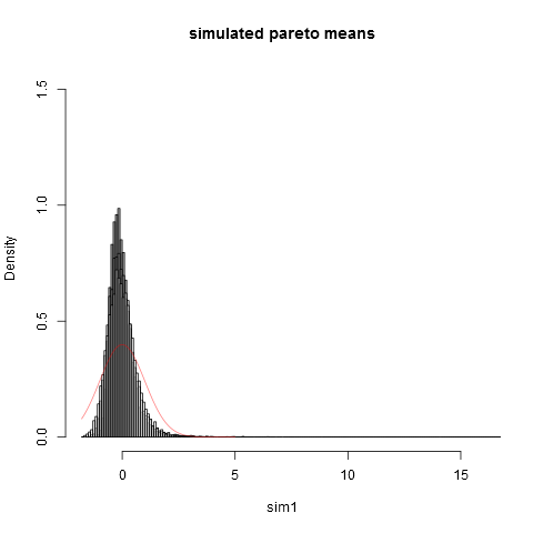
I will add an answer showing how bad the approximation from the central limit theorem (CLT) can be for the paretoPareto distribution, even in a case where the assumptions for CLT is fulfilled. The assumption is that there must be a finite variance, which for the paretoPareto means that $\alpha > 2$. For a more theoretical discussion of why this is so, see my answer here: What is the difference between finite and infinite variance
I will simulate data from the paretoPareto distribution with parameter $\alpha=2.1$, so that the variance "just barely exists". Redo my simulations with $\alpha=3.1$ to see the difference! Here is some R code:
### Pareto dist and the central limit theorem
###
require(actuar) # for (dpqr)pareto1()
require(MASS) # for Scott()
require(scales) # for alpha()
# We use (dpqr)pareto1(x,alpha,1)
#
alpha <- 2.1 # variance just barely exist
E <- function(alpha) ifelse(alpha <= 1,Inf,alpha/(alpha-1))
VAR <- function(alpha) ifelse(alpha <= 2,Inf,alpha/((alpha-1)^2 * (alpha-2)))
R <- 10000
e <- E(alpha)
sigma <- sqrt(VAR(alpha))
sim <- function(n) {
replicate(R, {x <- rpareto1(n,alpha,1)
x <- x-e
mean(x)*sqrt(n)/sigma },simplify=TRUE)
}
sim1 <- sim(10)
sim2 <- sim(100)
sim3 <- sim(1000)
sim4 <- sim(10000) # do take some time ...
### These are standardized so have all theoretically variance 1.
### But due to the long tail, the empirical variances are (surprisingly!) much lower:
sd(sim1)
sd(sim2)
sd(sim3)
sd(sim4)
### Now we plot the histograms:
hist(sim1,prob=TRUE,breaks="Scott",col=alpha("grey05",0.95),main="simulated pareto means",xlim=c(-1.8,16))
hist(sim2,prob=TRUE,breaks="Scott",col=alpha("grey30",0.5),add=TRUE)
hist(sim3,prob=TRUE,breaks="Scott",col=alpha("grey60",0.5),add=TRUE)
hist(sim4,prob=TRUE,breaks="Scott",col=alpha("grey90",0.5),add=TRUE)
plot(dnorm,from=-1.8,to=5,col=alpha("red",0.5),add=TRUE)
###  Pareto dist and the central limit theorem
    ###
    require(actuar) # for (dpqr)pareto1()
    require(MASS) #  for Scott()
    require(scales) # for alpha()
    # We use (dpqr)pareto1(x,alpha,1)
    #
    alpha <- 2.1  #  variance just barely exist
    E <-  function(alpha) ifelse(alpha <= 1,Inf,alpha/(alpha-1))
    VAR <- function(alpha) ifelse(alpha <= 2, Inf,
            alpha/((alpha-1)^2 * (alpha-2)))

    R <- 10000
    e <-  E(alpha)
    sigma  <-  sqrt(VAR(alpha))
    sim <-  function(n) {
        replicate(R, {x <- rpareto1(n,alpha,1)
            x <- x-e
            mean(x)*sqrt(n)/sigma },simplify=TRUE)
    }
    sim1 <- sim(10)
    sim2 <- sim(100)
    sim3 <- sim(1000)
    sim4 <- sim(10000) # do take some time ...

    ### These are standardized so have all
    ### theoretically variance 1.
    ### But due to the long tail, the empirical variances are
    ### (surprisingly!) much lower:

    sd(sim1)
    sd(sim2)
    sd(sim3)
    sd(sim4)

    ### Now we plot the histograms:
    hist(sim1, prob=TRUE, breaks="Scott", col=alpha("grey05",
    0.95), main="simulated Pareto means", xlim=c(-1.8,16))
    hist(sim2, prob=TRUE, breaks="Scott", col=alpha("grey30",
          0.5), add=TRUE)
    hist(sim3, prob=TRUE, breaks="Scott", col=alpha("grey60",
          0.5), add=TRUE)
    hist(sim4, prob=TRUE, breaks="Scott", col=alpha("grey90",
          0.5), add=TRUE)
    plot(dnorm, from=-1.8, to=5, col=alpha("red", 0.5), add=TRUE)


One can see that even at sample size $n=10000$ we are far away from the normal approximation. That the empirical variances are so much lower than the true theoretical variance $\sigma^2=1$ is due to the fact that we have a very large contribution to the variance from parts of the distribution in the extreme right tail that do not show up in most samples. This is to be expected always, when the variance "just barely exists". A practical way to think about that is the following. Pareto distributions is often proposed to model distributions of income (or wealth). The expectation of income (or wealth) will have a very large contribution from the very few billionaresbillionaires. Sampling with practical sample sizes will have a very small probability of including any billionaresbillionaires in the sample!

