Define $F(n, k)$ to be the number of ways to allocate $k$ options to $n$ flips such that each option appears either 0 or $\geq 2$ times. Then the probability that you see exactly $y$ unique values when you roll a $k$-sided dice $n$ times is:
$$ Pr(Y=y) = \frac{{k\choose y}{n\choose y}y!F(n-y, k-y)}{k^n} $$
Basically, there are ${k \choose y}$ ways to select the $y$ unique options from all $k$ options, ${n\choose y}$ ways to select the $y$ rolls for these unique options, and $y!$ orderings of the $y$ options within these rolls.
All that remains is to compute $F(n, k)$. There are a few simple cases and then a recursive definition:
\begin{align*} F(0, k) &= 1 &\forall~k\geq 0 \\ F(1, k) &= 0 &\forall~k\geq 0 \\ F(n, 0) &= 0 &\forall~n\geq 1 \\ F(n, k) &= F(n, k-1) + \sum_{i=2}^n {n\choose i}F(n-i, k-1) &\forall~n\geq 2, k\geq 1 \end{align*}
The recursive step selects an arbitrary option and separately considers the number of allocations for which it appears $0, 2, 3, \ldots, n$ times. This formulation enables the calculation of the entire pmf in $O(n^2k)$ runtime, which should be a good deal more efficient than summing over all valid partitions of the multinomial distribution. Here's an R implementation:
uniquePMF <- function(n, k) {
  F <- matrix(0, nrow=n+1, ncol=k+1)
  F[1,] <- 1
  for (.k in 1:k) {
    for (.n in 2:n) {
      F[.n+1,.k+1] <- F[.n+1,.k] + sum(choose(.n, 2:.n)*F[.n-(2:.n)+1,.k])
    }
  }
  out <- sapply(0:min(n, k), function(y) choose(k, y)*choose(n, y)*factorial(y)*F[n-y+1,k-y+1]) / k^n
  names(out) <- 0:min(n, k)
  out
}
This returns your hand-calculated results for the $n=2, k=3$ case:
uniquePMF(2, 3)
#         0         1         2
# 0.3333333 0.0000000 0.6666667
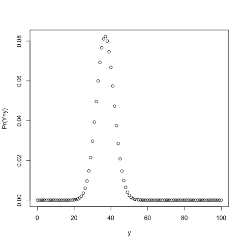
It can also comfortably handle larger instances (here $n=k=100$):
plot(0:100, uniquePMF(10100, 10100)
#          0          1          2          3          4          5          6
# 0.00811639 0.04794633 0.14082336 0.21089376 0.27052704 0.15621984 0.12700800
#          7          8          9         10
# 0.02177280 0.01632960, 0.00000000xlab="y", 0.00036288ylab="Pr(Y=y)")

