Summary: The trick appears to be a Bayesian approach which assumes a uniform (Jeffreys) prior for the hidden parameter ($z_\mu$ in appendix B of the paper, $\theta$ here).
I believe there may be a Bayesian-style approach to get the equations given in the paper's appendix B.
As I understand it, the experiment boils down to a statistic $z\sim\mathrm{N}_{\theta,1}$. The mean $\theta$ of the sampling distribution is unknown, but vanishes under the null hypothesis, $\theta\mid{}H_0=0$.
Call the experimentally observed statistic $\hat{z}\mid\theta\sim\mathrm{N}_{\theta,1}$. Then if we assume a "uniform" (improper) prior on $\theta\sim1$, the Bayesian posterior is $\theta\mid\hat{z}\sim\mathrm{N}_{\hat{z},1}$. If we then update the original sampling distribution by marginalizing over $\theta\mid\hat{z}$, the posterior becomes $z\mid\hat{z}\sim\mathrm{N}_{\hat{z},2}$. (The doubled variance is due to convolution of Gaussians.)
Mathematically at least, this seems to work. And it explains how the $\frac{1}{\sqrt{2}}$ factor "magically" appears going from equation B2 to equation B3.
Discussion
How can this result be reconciled with the standard null hypothesis testing framework? One possible interpretation is as follows.
In the standard framework, the null hypothesis is in some sense the "default" (e.g. we speak of "rejecting the null"). In the above Bayesian context this would be a non-uniform prior that prefers $\theta=0$. If we take this to be $\theta\sim\mathrm{N}_{0,\lambda^2}$, then the variance $\lambda^2$ represents our prior uncertainty.
Carrying this prior through the analysis above, we find $$\theta\sim\mathrm{N}_{0,\lambda^2} \implies \theta\mid\hat{z}\sim\mathrm{N}_{\delta^2\hat{z},\delta^2} \,,\, z\mid\hat{z}\sim\mathrm{N}_{\delta^2\hat{z},1+\delta^2} \,,\, \delta^2\equiv\tfrac{1}{1+\lambda^{-2}}\in[0,1]$$ From this we can see that in the limit $\lambda\to\infty$ we recover the analysis above. But in the limit $\lambda\to{0}$ our "posteriors" become the null, $\theta\mid\hat{z}\sim\mathrm{N}_{0,0}$ and $z\mid\hat{z}\sim\mathrm{N}_{0,1}$, so we recover the standard result, ${p}\mid{\hat{z}}\sim\mathrm{U}_{0,1}$.
(For repeated studies, the above suggests an interesting question here about the implications for Bayesian updating vs. "traditional" methods for meta-analysis. I am completely ignorant on the subject of meta-analysis though!)
Appendix
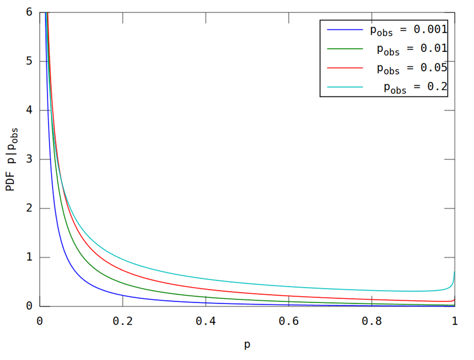
As requested in the comments, here is a plot for comparison. This is a relatively straightforward application of the formulas in the paper. However I will write these out to ensure no ambiguity.
Let $p$ denote the one-sided p value for the statistic $z$, and denote its (posterior) CDF by $F[u]\equiv\Pr\big[\,p\leq{u}\mid{\hat{z}}\,\big]$. Then equation B3 from the appendix is equivalent to $$F[p]=1-\Phi\left[\tfrac{1}{\sqrt{2}}\left(z[p]-\hat{z}\right)\right] \,,\, z[p]=\Phi^{-1}[1-p]$$ where $\Phi[\,\,]$ is the standard normal CDF. The corresponding density is then $$f\big[p\big]\equiv{F^\prime}\big[p\big]=\frac{\phi\Big[(z-\hat{z})/\sqrt{2}\,\Big]}{\sqrt{2}\,\phi\big[z\big]}$$ where $\phi[\,\,]$ is the standard normal PDF, and $z=z[p]$ as in the CDF formula. Finally, if we denote by $\hat{p}$ the observed two-sided p value corresponding to $\hat{z}$, then we have $$\hat{z}=\Phi^{-1}\Big[1-\tfrac{\hat{p}}{2}\Big]$$
Using these equations gives the figure below, which should be comparable to the paper's figure 5 quoted in the question.

(This was produced by the following Matlab code; run here.)
phat2=[1e-3,1e-2,5e-2,0.2]'; zhat=norminv(1-phat2/2);
np=1e3+1; p1=(1:np)/(np+1); z=norminv(1-p1);
p1pdf=normpdf((z-zhat)/sqrt(2))./(sqrt(2)*normpdf(z));
plot(p1,p1pdf,'LineWidth',1); axis([0,1,0,6]);
xlabel('p'); ylabel('PDF p|p_{obs}');
legend(arrayfun(@(p)sprintf('p_{obs} = %g',p),phat2,'uni',0));
