Biggest change is adding comment to warn about the one possible danger of starting with an initial value greater than the desired root. Added some other expository tweaks.
Source Link
cardinal
  • 27.3k
  • 8
  • 105
  • 140

Property 1: The function $\df$ is convex and decreasing on $\lambda \geq 0$. (Take derivatives.)
Consequence 1(a): Newton's root-finding algorithm will behave very nicely in this situation. Let $y$ be the desired degrees of freedom and $\lambda_0$ the corresponding root, i.e., $y = \df(\lambda_0)$. In particular, if we start out with any initial value $\lambda_1$ such that$\lambda_1 < \lambda_0$ (so, $\df(\lambda_1) > y$), then the sequence of Newton-step iterations $\lambda_1,\lambda_2,\ldots$ will converge monotonically to the unique solution $\lambda_0$.
Consequence 1(b): Furthermore, if we were to start out with $\df(\lambda_1) < y$$\lambda_1 > \lambda_0$, then the first step would yield $\lambda_2$ such that $\df(\lambda_2) > y$ and, then$\lambda_2 \leq \lambda_0$, from thereonwhence it will monotonically increase to the solution. by the previous consequence (Intuitivelysee caveat below). Intuitively, this last fact follows because if we start onto the right of the root, the derivative is "too" shallow due to the convexity of $\df$ and so the first Newton step will take us somewhere to the left of the root.) NB Since $\df$ is not in general convex for negative $\lambda$, this provides a strong reason to prefer starting to the left of the desired root. Otherwise, we need to double check that the Newton step hasn't resulted in a negative value for the estimated root, which may place us somewhere in a nonconvex portion of $\df$.
Consequence 1(bc): Once we've found the root for some $y_1$ and are then searching for the root from some $y_2 < y_1$, using $\lambda_1$ such that $\df(\lambda_1) = y_1$ as our initial guess guarantees we start to the left of the second root. So, our convergence is guaranteed to be monotonic from there.

Property 2: Reasonable bounds exist to give "safe" starting points. Using convexity arguments and Jensen's inequality, we have the following bounds $$ \frac{p}{1+ \frac{\lambda}{p}\sum d_i^{-2}} \leq \df(\lambda) \leq \frac{p \sum_i d_i^2}{\sum_i d_i^2 + p \lambda} \>. $$ Consequence 2: This tells us that the root $\lambda_0$ satisfying $\df(\lambda_0) = y$ obeys $$ \frac{1}{\frac{1}{p}\sum_i d_i^{-2}}\left(\frac{p - y}{y}\right) \leq \lambda_0 \leq \left(\frac{1}{p}\sum_i d_i^2\right) \left(\frac{p - y}{y}\right) \>. \tag{$\star$} $$ So, up to a common constant, we've sandwiched the root in between the harmonic and arithmetic means of the $d_i^2$.

A very efficient algorithm given a grid of desired degrees of freedom $y_1, \ldots y_n$ in $(0,p]$ is to sort them in decreasing order and then sequentially find the root of each, using the previous root as the starting point for the following one. We can refine this further by checking if each root is to the right ofgreater than the lower bound for the next root, and, if not, we can start the next iteration at the lower bound instead.

# Newton's step for finding solutions to regularization dof.

dof <- function(lambda, d) { sum(1/(1+lambda / (d[d>0])^2)) }
dof.prime <- function(lambda, d) { -sum(1/(d[d>0]+lambda / d[d>0])^2) }

newton.step <- function(lambda, y, d)
{ lambda - (dof(lambda,d)-y)/dof.prime(lambda,d) }

# Full Newton step; Finds the root of y = dof(lambda, d).
newton <- function(y, d, lambda = NA, tol=1e-10, smart.start=T)
{
    if( is.na(lambda) || smart.start )
        lambda <- max(ifelse(is.na(lambda),0,lambda), (sum(d>0)/y-1)/mean(1/(d[d>0])^2))
    iter <- 0
    yn   <- Inf
    while( abs(y-yn) > tol )
    {
        lambda <- max(0, newton.step(lambda, y, d)) # max = pedantically safe
        yn <- dof(lambda,d)
        iter = iter + 1
    }
    return(list(lambda=lambda, dof=y, iter=iter, err=abs(y-yn)))
}

Property 1: The function $\df$ is convex and decreasing on $\lambda \geq 0$. (Take derivatives.)
Consequence 1(a): Newton's root-finding algorithm will behave very nicely in this situation. In particular, if we start out with any initial value $\lambda_1$ such that $\df(\lambda_1) > y$, then the sequence of Newton-step iterations will converge monotonically to the unique solution. Furthermore, if we were to start out with $\df(\lambda_1) < y$, then the first step would yield $\lambda_2$ such that $\df(\lambda_2) > y$ and, then, from thereon it will monotonically increase to the solution. (Intuitively, this last fact follows because if we start on the right of the root, the derivative is "too" shallow and so the first Newton step will take us somewhere to the left of the root.)
Consequence 1(b): Once we've found the root for some $y_1$ and are then searching for the root from some $y_2 < y_1$, using $\lambda_1$ such that $\df(\lambda_1) = y_1$ as our initial guess guarantees we start to the left of the second root. So, our convergence is guaranteed to be monotonic from there.

Property 2: Reasonable bounds exist to give "safe" starting points. Using convexity arguments and Jensen's inequality, we have the following bounds $$ \frac{p}{1+ \frac{\lambda}{p}\sum d_i^{-2}} \leq \df(\lambda) \leq \frac{p \sum_i d_i^2}{\sum_i d_i^2 + p \lambda} \>. $$ Consequence 2: This tells us that the root $\lambda_0$ satisfying $\df(\lambda_0) = y$ obeys $$ \frac{1}{\frac{1}{p}\sum_i d_i^{-2}}\left(\frac{p - y}{y}\right) \leq \lambda_0 \leq \left(\frac{1}{p}\sum_i d_i^2\right) \left(\frac{p - y}{y}\right) \>. \tag{$\star$} $$ So, up to a constant, we've sandwiched the root in between the harmonic and arithmetic means of the $d_i^2$.

A very efficient algorithm given a grid of desired degrees of freedom $y_1, \ldots y_n$ in $(0,p]$ is to sort them in decreasing order and then sequentially find the root of each, using the previous root as the starting point for the following one. We can refine this further by checking if each root is to the right of the lower bound for the next root, and, if not, we can start the next iteration at the lower bound instead.

# Newton's step for finding solutions to regularization dof.

dof <- function(lambda, d) { sum(1/(1+lambda / (d[d>0])^2)) }
dof.prime <- function(lambda, d) { -sum(1/(d[d>0]+lambda / d[d>0])^2) }

newton.step <- function(lambda, y, d)
{ lambda - (dof(lambda,d)-y)/dof.prime(lambda,d) }

# Full Newton step; Finds the root of y = dof(lambda, d).
newton <- function(y, d, lambda = NA, tol=1e-10, smart.start=T)
{
    if( is.na(lambda) || smart.start )
        lambda <- max(ifelse(is.na(lambda),0,lambda), (sum(d>0)/y-1)/mean(1/(d[d>0])^2))
    iter <- 0
    yn   <- Inf
    while( abs(y-yn) > tol )
    {
        lambda <- newton.step(lambda, y, d)
        yn <- dof(lambda,d)
        iter = iter + 1
    }
    return(list(lambda=lambda, dof=y, iter=iter, err=abs(y-yn)))
}
Property 1: The function $\df$ is convex and decreasing on $\lambda \geq 0$. (Take derivatives.)
Consequence 1(a): Newton's root-finding algorithm will behave very nicely in this situation. Let $y$ be the desired degrees of freedom and $\lambda_0$ the corresponding root, i.e., $y = \df(\lambda_0)$. In particular, if we start out with any initial value $\lambda_1 < \lambda_0$ (so, $\df(\lambda_1) > y$), then the sequence of Newton-step iterations $\lambda_1,\lambda_2,\ldots$ will converge monotonically to the unique solution $\lambda_0$.
Consequence 1(b): Furthermore, if we were to start out with $\lambda_1 > \lambda_0$, then the first step would yield $\lambda_2 \leq \lambda_0$, from whence it will monotonically increase to the solution by the previous consequence (see caveat below). Intuitively, this last fact follows because if we start to the right of the root, the derivative is "too" shallow due to the convexity of $\df$ and so the first Newton step will take us somewhere to the left of the root. NB Since $\df$ is not in general convex for negative $\lambda$, this provides a strong reason to prefer starting to the left of the desired root. Otherwise, we need to double check that the Newton step hasn't resulted in a negative value for the estimated root, which may place us somewhere in a nonconvex portion of $\df$.
Consequence 1(c): Once we've found the root for some $y_1$ and are then searching for the root from some $y_2 < y_1$, using $\lambda_1$ such that $\df(\lambda_1) = y_1$ as our initial guess guarantees we start to the left of the second root. So, our convergence is guaranteed to be monotonic from there.

Property 2: Reasonable bounds exist to give "safe" starting points. Using convexity arguments and Jensen's inequality, we have the following bounds $$ \frac{p}{1+ \frac{\lambda}{p}\sum d_i^{-2}} \leq \df(\lambda) \leq \frac{p \sum_i d_i^2}{\sum_i d_i^2 + p \lambda} \>. $$ Consequence 2: This tells us that the root $\lambda_0$ satisfying $\df(\lambda_0) = y$ obeys $$ \frac{1}{\frac{1}{p}\sum_i d_i^{-2}}\left(\frac{p - y}{y}\right) \leq \lambda_0 \leq \left(\frac{1}{p}\sum_i d_i^2\right) \left(\frac{p - y}{y}\right) \>. \tag{$\star$} $$ So, up to a common constant, we've sandwiched the root in between the harmonic and arithmetic means of the $d_i^2$.

A very efficient algorithm given a grid of desired degrees of freedom $y_1, \ldots y_n$ in $(0,p]$ is to sort them in decreasing order and then sequentially find the root of each, using the previous root as the starting point for the following one. We can refine this further by checking if each root is greater than the lower bound for the next root, and, if not, we can start the next iteration at the lower bound instead.

# Newton's step for finding solutions to regularization dof.

dof <- function(lambda, d) { sum(1/(1+lambda / (d[d>0])^2)) }
dof.prime <- function(lambda, d) { -sum(1/(d[d>0]+lambda / d[d>0])^2) }

newton.step <- function(lambda, y, d)
{ lambda - (dof(lambda,d)-y)/dof.prime(lambda,d) }

# Full Newton step; Finds the root of y = dof(lambda, d).
newton <- function(y, d, lambda = NA, tol=1e-10, smart.start=T)
{
    if( is.na(lambda) || smart.start )
        lambda <- max(ifelse(is.na(lambda),0,lambda), (sum(d>0)/y-1)/mean(1/(d[d>0])^2))
    iter <- 0
    yn   <- Inf
    while( abs(y-yn) > tol )
    {
        lambda <- max(0, newton.step(lambda, y, d)) # max = pedantically safe
        yn <- dof(lambda,d)
        iter = iter + 1
    }
    return(list(lambda=lambda, dof=y, iter=iter, err=abs(y-yn)))
}
Caught an ugly bug in my code; Fixing it actually reduces the number of Newton steps a bit from the previous version of the table.
Source Link
cardinal
  • 27.3k
  • 8
  • 105
  • 140
# Table of Newton iterations per root.
# Without using lower-bound check.
  1  3  4  5  6 
  1 28 65  5  1 
# Table with lower-bound check.
  1  32  43 
  1 2814 7185 
# Newton's step for finding solutions to regularization dof.

dof <- function(lambda, d) { sum(1/(1+lambda / (d[d>0])^2)) }
dof.prime <- function(lambda, d) { -sum(1/(d[d>0]+lambda / d[d>0])^2) }

newton.step <- function(lambda, y, d)
{ lambda - (dof(lambda,d)-y)/dof.prime(lambda,d) }

# Full Newton step; Finds the root of y = dof(lambda, d).
newton <- function(y, d, lambda = NA, tol=1e-10, smart.start=T)
{
    if( is.na(lambda) || smart.start )
        lambda <- max(ifelse(is.na(lambda),0,lambda), (sum(d>0)/y-1)/mean(1/(d[d>0])^2))
    iter <- 0
    yn   <- Inf
    while( abs(y-yn) > tol )
    {
        lambda <- newton.step(lambda, y, d)
        yn <- dof(lambda,d)
        iter = iter + 1
    }
    return(list(lambda=lambda, dof=y, iter=iter, err=abs(y-yn), root=y))
}
# Table of Newton iterations per root.
# Without using lower-bound check.
  1  3  4  5  6 
  1 28 65  5  1 
# Table with lower-bound check.
  1  3  4 
  1 28 71 
# Newton's step for finding solutions to regularization dof.

dof <- function(lambda, d) { sum(1/(1+lambda / (d[d>0])^2)) }
dof.prime <- function(lambda, d) { -sum(1/(d[d>0]+lambda / d[d>0])^2) }

newton.step <- function(lambda, y, d)
{ lambda - (dof(lambda,d)-y)/dof.prime(lambda,d) }

# Full Newton step; Finds the root of y = dof(lambda, d).
newton <- function(y, d, lambda = NA, tol=1e-10, smart.start=T)
{
    if( is.na(lambda) || smart.start )
        lambda <- max(ifelse(is.na(lambda),0,lambda), (sum(d>0)/y-1)/mean(1/d[d>0]))
    iter <- 0
    yn   <- Inf
    while( abs(y-yn) > tol )
    {
        lambda <- newton.step(lambda, y, d)
        yn <- dof(lambda,d)
        iter = iter + 1
    }
    return(list(lambda=lambda, iter=iter, err=abs(y-yn), root=y))
}
# Table of Newton iterations per root.
# Without using lower-bound check.
  1  3  4  5  6 
  1 28 65  5  1 
# Table with lower-bound check.
  1  2  3 
  1 14 85 
# Newton's step for finding solutions to regularization dof.

dof <- function(lambda, d) { sum(1/(1+lambda / (d[d>0])^2)) }
dof.prime <- function(lambda, d) { -sum(1/(d[d>0]+lambda / d[d>0])^2) }

newton.step <- function(lambda, y, d)
{ lambda - (dof(lambda,d)-y)/dof.prime(lambda,d) }

# Full Newton step; Finds the root of y = dof(lambda, d).
newton <- function(y, d, lambda = NA, tol=1e-10, smart.start=T)
{
    if( is.na(lambda) || smart.start )
        lambda <- max(ifelse(is.na(lambda),0,lambda), (sum(d>0)/y-1)/mean(1/(d[d>0])^2))
    iter <- 0
    yn   <- Inf
    while( abs(y-yn) > tol )
    {
        lambda <- newton.step(lambda, y, d)
        yn <- dof(lambda,d)
        iter = iter + 1
    }
    return(list(lambda=lambda, dof=y, iter=iter, err=abs(y-yn)))
}
Source Link
cardinal
  • 27.3k
  • 8
  • 105
  • 140

This is a long answer. So, let's give a short-story version of it here.

  • There's no nice algebraic solution to this root-finding problem, so we need a numerical algorithm.
  • The function $\mathrm{df}(\lambda)$ has lots of nice properties. We can harness these to create a specialized version of Newton's method for this problem with guaranteed monotonic convergence to each root.
  • Even brain-dead R code absent any attempts at optimization can compute a grid of size 100 with $p = 100\,000$ in a few of seconds. Carefully written C code would reduce this by at least 2–3 orders of magnitude.

There are two schemes given below to guarantee monotonic convergence. One uses bounds shown below, which seem to help save a Newton step or two on occasion.

Example: $p = 100\,000$ and a uniform grid for the degrees of freedom of size 100. The eigenvalues are Pareto-distributed, hence highly skewed. Below are tables of the number of Newton steps to find each root.

# Table of Newton iterations per root.
# Without using lower-bound check.
  1  3  4  5  6 
  1 28 65  5  1 
# Table with lower-bound check.
  1  3  4 
  1 28 71 

There won't be a closed-form solution for this, in general, but there is a lot of structure present which can be used to produce very effective and safe solutions using standard root-finding methods.

Before digging too deeply into things, let's collect some properties and consequences of the function $$\newcommand{\df}{\mathrm{df}} \df(\lambda) = \sum_{i=1}^p \frac{d_i^2}{d_i^2 + \lambda} \>. $$

Property 0: $\df$ is a rational function of $\lambda$. (This is apparent from the definition.)
Consequence 0: No general algebraic solution will exist for finding the root $\df(\lambda) - y = 0$. This is because there is an equivalent polynomial root-finding problem of degree $p$ and so if $p$ is not extremely small (i.e., less than five), no general solution will exist. So, we'll need a numerical method.

Property 1: The function $\df$ is convex and decreasing on $\lambda \geq 0$. (Take derivatives.)
Consequence 1(a): Newton's root-finding algorithm will behave very nicely in this situation. In particular, if we start out with any initial value $\lambda_1$ such that $\df(\lambda_1) > y$, then the sequence of Newton-step iterations will converge monotonically to the unique solution. Furthermore, if we were to start out with $\df(\lambda_1) < y$, then the first step would yield $\lambda_2$ such that $\df(\lambda_2) > y$ and, then, from thereon it will monotonically increase to the solution. (Intuitively, this last fact follows because if we start on the right of the root, the derivative is "too" shallow and so the first Newton step will take us somewhere to the left of the root.)
Consequence 1(b): Once we've found the root for some $y_1$ and are then searching for the root from some $y_2 < y_1$, using $\lambda_1$ such that $\df(\lambda_1) = y_1$ as our initial guess guarantees we start to the left of the second root. So, our convergence is guaranteed to be monotonic from there.

Property 2: Reasonable bounds exist to give "safe" starting points. Using convexity arguments and Jensen's inequality, we have the following bounds $$ \frac{p}{1+ \frac{\lambda}{p}\sum d_i^{-2}} \leq \df(\lambda) \leq \frac{p \sum_i d_i^2}{\sum_i d_i^2 + p \lambda} \>. $$ Consequence 2: This tells us that the root $\lambda_0$ satisfying $\df(\lambda_0) = y$ obeys $$ \frac{1}{\frac{1}{p}\sum_i d_i^{-2}}\left(\frac{p - y}{y}\right) \leq \lambda_0 \leq \left(\frac{1}{p}\sum_i d_i^2\right) \left(\frac{p - y}{y}\right) \>. \tag{$\star$} $$ So, up to a constant, we've sandwiched the root in between the harmonic and arithmetic means of the $d_i^2$.

This assumes that $d_i > 0$ for all $i$. If this is not the case, then the same bound holds by considering only the positive $d_i$ and replacing $p$ by the number of positive $d_i$. NB: Since $\df(0) = p$ assuming all $d_i > 0$, then $y \in (0,p]$, whence the bounds are always nontrivial (e.g., the lower bound is always nonnegative).

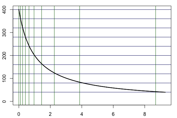
Here is a plot of a "typical" example of $\df(\lambda)$ with $p = 400$. We've superimposed a grid of size 10 for the degrees of freedom. These are the horizontal lines in the plot. The vertical green lines correspond to the lower bound in $(\star)$.

Example dof plot with grid and bounds

An algorithm and some example R code

A very efficient algorithm given a grid of desired degrees of freedom $y_1, \ldots y_n$ in $(0,p]$ is to sort them in decreasing order and then sequentially find the root of each, using the previous root as the starting point for the following one. We can refine this further by checking if each root is to the right of the lower bound for the next root, and, if not, we can start the next iteration at the lower bound instead.

Here is some example code in R, with no attempts made to optimize it. As seen below, it is still quite fast even though R is—to put it politely—horrifingly, awfully, terribly slow at loops.

# Newton's step for finding solutions to regularization dof.

dof <- function(lambda, d) { sum(1/(1+lambda / (d[d>0])^2)) }
dof.prime <- function(lambda, d) { -sum(1/(d[d>0]+lambda / d[d>0])^2) }

newton.step <- function(lambda, y, d)
{ lambda - (dof(lambda,d)-y)/dof.prime(lambda,d) }

# Full Newton step; Finds the root of y = dof(lambda, d).
newton <- function(y, d, lambda = NA, tol=1e-10, smart.start=T)
{
    if( is.na(lambda) || smart.start )
        lambda <- max(ifelse(is.na(lambda),0,lambda), (sum(d>0)/y-1)/mean(1/d[d>0]))
    iter <- 0
    yn   <- Inf
    while( abs(y-yn) > tol )
    {
        lambda <- newton.step(lambda, y, d)
        yn <- dof(lambda,d)
        iter = iter + 1
    }
    return(list(lambda=lambda, iter=iter, err=abs(y-yn), root=y))
}

Below is the final full algorithm which takes a grid of points, and a vector of the $d_i$ (not $d_i^2$!).

newton.grid <- function(ygrid, d, lambda=NA, tol=1e-10, smart.start=TRUE)
{
    p <- sum(d>0)
    if( any(d < 0) || all(d==0) || any(ygrid > p) 
        || any(ygrid <= 0) || (!is.na(lambda) && lambda < 0) )
        stop("Don't try to fool me. That's not nice. Give me valid inputs, please.")
    ygrid <- sort(ygrid, decreasing=TRUE)
    out    <- data.frame()
    lambda <- NA
    for(y in ygrid)
    {
        out <- rbind(out, newton(y,d,lambda, smart.start=smart.start))
        lambda <- out$lambda[nrow(out)]
    }
    out
}

Sample function call

set.seed(17)
p <- 100000
d <- sqrt(sort(exp(rexp(p, 10)),decr=T))
ygrid <- p*(1:100)/100
# Should take ten seconds or so.
out <- newton.grid(ygrid,d)