Return to Answer

library(mlr)
daf = read.csv("https://pastebin.com/raw/p1cCCYBR", sep = " ", header = FALSE)

tsk = list(
  tsk1110 = makeRegrTask(id = "tsk1110", data = daf, target = colnames(daf)[1]),
  tsk500 = makeRegrTask(id = "tsk500", data = daf[, c(1,sample(ncol(daf)-1, 500)+1)], target = colnames(daf)[1]),
  tsk100 = makeRegrTask(id = "tsk100", data = daf[, c(1,sample(ncol(daf)-1, 100)+1)], target = colnames(daf)[1]),
  tsk50 = makeRegrTask(id = "tsk50", data = daf[, c(1,sample(ncol(daf)-1, 50)+1)], target = colnames(daf)[1]),
  tsk10 = makeRegrTask(id = "tsk10", data = daf[, c(1,sample(ncol(daf)-1, 10)+1)], target = colnames(daf)[1])
)

lrn = makeLearner("regr.glmnet", alpha = 0)
rdesc = makeResampleDesc("CV", iters = 10)
msrs = list(mse, rsq)
ctrl = makeTuneControlGrid(resolution = 15L)
pset = makeParamSet( makeNumericParam("lambda", lower = -10, upper = 10, trafo = function(x) exp(x)))
cvl = makeTuneWrapper(learner = lrn, resampling = rdesc, measures = msrs, control = ctrl, par.set = pset)
bm = benchmark(learners = cvl, tasks = tsk, resamplings = rdesc, measures = msrs)

> bm
  task.id        learner.id mse.test.mean rsq.test.mean
1   tsk10 regr.glmnet.tuned     0.9029739   -0.34385207
2  tsk100 regr.glmnet.tuned     0.9860033   -0.20159950
3 tsk1110 regr.glmnet.tuned     0.6836474    0.08630208
4   tsk50 regr.glmnet.tuned     0.9159190   -0.15177725
5  tsk500 regr.glmnet.tuned     0.8874529    0.04095012

They basically got the same slightly better than random performance, but glmnet is good enough to squeeze some information the more features you feed it.

getBMRTuneResults(bm, as.df = TRUE, task.ids = "tsk1110")
#   task.id        learner.id iter   lambda mse.test.mean rsq.test.mean
#1  tsk1110 regr.glmnet.tuned    1 0.239651     0.7234743    0.06932993
#2  tsk1110 regr.glmnet.tuned    2 0.239651     0.6318552    0.10130075
#3  tsk1110 regr.glmnet.tuned    3 0.239651     0.7202225    0.09277869
#4  tsk1110 regr.glmnet.tuned    4 4.172734     0.7169810   -0.08232901
#5  tsk1110 regr.glmnet.tuned    5 0.239651     0.7163615   -0.05643168
#6  tsk1110 regr.glmnet.tuned    6 0.239651     0.6655465    0.13894617
#7  tsk1110 regr.glmnet.tuned    7 0.239651     0.7125394    0.14249063
#8  tsk1110 regr.glmnet.tuned    8 0.239651     0.7312063   -0.56975408
#9  tsk1110 regr.glmnet.tuned    9 0.239651     0.6895064   -0.03308516
#10 tsk1110 regr.glmnet.tuned   10 0.239651     0.6370360    0.02805295

Notice the lambdas are already transformed. Not a single fold picked the minimal lambda $\exp(-10)\approx 4.54 \mathbf E-5$ (this is the same behavior with cv.glmnet in R).

So, basically, $\lambda>0$ really improves the fit.

We picked the best lambda in the most parsimonious way, and we expect it to be the more performant than any other arbitrary selection. Repeating the benchmark with the addition of a glmnet with lambda set to a ludicrously small value (1E-100), we see that our tuning really improves the result.

bm2 = benchmark(learners = list(cvl, makeLearner("regr.glmnet", alpha = 0, lambda = 1E-100)), tasks = tsk, resamplings = rdesc, measures = msrs)
getBMRAggrPerformances(bm2, as.df = TRUE)
#   task.id        learner.id mse.test.mean rsq.test.mean
#1    tsk10 regr.glmnet.tuned     1.0302354   -0.36840610
#2    tsk10       regr.glmnet     1.2542921   -0.58709603
#3   tsk100 regr.glmnet.tuned     0.8721003   -0.01025020
#4   tsk100       regr.glmnet     2.6139448   -2.56834215
#5  tsk1110 regr.glmnet.tuned     0.6716137    0.26026566
#6  tsk1110       regr.glmnet     1.4569493   -0.76811536
#7    tsk50 regr.glmnet.tuned     0.7851516    0.02185949
#8    tsk50       regr.glmnet     1.8970910   -1.69729756
#9   tsk500 regr.glmnet.tuned     0.8556580   -0.05821649
#10  tsk500       regr.glmnet     1.6703070   -1.02238746

There's an element of randomness involved, but the tuned model always outperform the asymptotically-OLS ridge, often by quite a marging.

library(mlr)
daf = read.csv("https://pastebin.com/raw/p1cCCYBR", sep = " ", header = FALSE)

tsk = list(
  tsk1110 = makeRegrTask(id = "tsk1110", data = daf, target = colnames(daf)[1]),
  tsk500 = makeRegrTask(id = "tsk500", data = daf[, c(1,sample(ncol(daf)-1, 500)+1)], target = colnames(daf)[1]),
  tsk100 = makeRegrTask(id = "tsk100", data = daf[, c(1,sample(ncol(daf)-1, 100)+1)], target = colnames(daf)[1]),
  tsk50 = makeRegrTask(id = "tsk50", data = daf[, c(1,sample(ncol(daf)-1, 50)+1)], target = colnames(daf)[1]),
  tsk10 = makeRegrTask(id = "tsk10", data = daf[, c(1,sample(ncol(daf)-1, 10)+1)], target = colnames(daf)[1])
)

rdesc = makeResampleDesc("CV", iters = 10)
msrs = list(mse, rsq)
configureMlr(on.par.without.desc = "quiet")
bm3 = benchmark(learners = list( 
    makeLearner("regr.cvglmnet", alpha = 0, lambda = c(0, exp(seq(-10, 10, length.out = 150))),
    makeLearner("regr.glmnet", alpha = 0, lambda = c(0, exp(seq(-10, 10, length.out = 150))), s = 151)
    ), tasks = tsk, resamplings = rdesc, measures = msrs)

getBMRAggrPerformances(bm3, as.df = TRUE)
#   task.id    learner.id mse.test.mean rsq.test.mean
#1    tsk10 regr.cvglmnet     1.0308055  -0.224534550
#2    tsk10   regr.glmnet     1.3685799  -0.669473387
#3   tsk100 regr.cvglmnet     0.7996823   0.031731316
#4   tsk100   regr.glmnet     1.3092522  -0.656879104
#5  tsk1110 regr.cvglmnet     0.8236786   0.009315037
#6  tsk1110   regr.glmnet     0.6866745   0.117540454
#7    tsk50 regr.cvglmnet     1.0348319  -0.188568886
#8    tsk50   regr.glmnet     2.5468091  -2.423461744
#9   tsk500 regr.cvglmnet     0.7210185   0.173851634
#10  tsk500   regr.glmnet     0.6171841   0.296530437

They do basically the same across tasks.

sapply(lapply(getBMRModels(bm3, task.ids = "tsk1110")[[1]][[1]], "[[", 2), "[[", "lambda.min")
# [1] 4.539993e-05 4.539993e-05 2.442908e-01 1.398738e+00 4.539993e-05
# [6] 0.000000e+00 4.539993e-05 3.195187e-01 2.793841e-01 4.539993e-05

Notice the lambdas are already transformed. Some fold even picked the minimal lambda $\lambda = 0$.

#EDIT: After comments by amoeba, it became clear the regularization path is an important step in the glmnet estimation, so the code now reflects it. This way, most discrepancies vanished.

So, basically, $\lambda>0$ really improves the fit (edit: but not by much!).

Edit: Keep in mind, though, the ridge regularization path makes use of previous parameter estimates when we call glmnet, but this is beyond my expertise. If we set a really low lambda in isolation, it'll likely degrade performance.

Edit: notice though when we set lambda to 0 after running the whole regularization path performance doesn't degrade as such, therefore the regularization path is key to understand what's going on!

Also, I don't quite understand your last line. Look at the cv.glmnet output for p=100. It will have very different shape. So what affects this shape (asymptote on the left vs. no asymptote) when p=100 or p=1000?

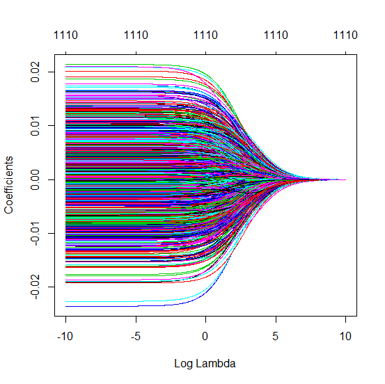
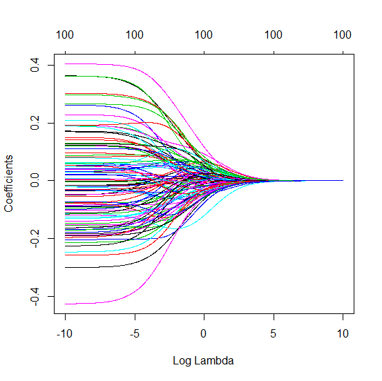
Let's compare the regularization paths for both:

fit1000 = glmnet(x, y, alpha = 0, lambda = exp(seq(-10,10, length.out = 1001)))
fit100 = glmnet(x[, sample(1000, 100)], y, alpha = 0, lambda = exp(seq(-10,10, length.out = 1001)))
plot(fit1000, "lambda")

x11()
plot(fit100, "lambda")

It becomes clear $p=1000$ affords larger coefficients at increasing $\lambda$, even though it has smaller coefficients for asymptotically-OLS ridge, at the left of both plots. So, basically, $p=100$ overfits at the left of the graph, and that probably explains the difference in behavior between them.

It's harder for $p=1000$ to overfit because, even though Ridge shrinks coefficients to zero, they are never reach zero. This mean that the predictive power of the model is shared between many more components, making it easier to predict around the mean instead of being carried away by noise.

#Comments

It seems you are getting a tiny minimum for some non-zero lambda (I am looking at your figure), but the curve is still really really flat to the left of it. So my main question remains as to why λ→0 does not noticeably overfit. I don't see an answer here yet. Do you expect this to be a general phenomenon? I.e. for any data with n≪p, lambda=0 will perform [almost] as good as optimal lambda? Or is it something special about these data? If you look above in the comments, you'll see that many people did not even believe me that it's possible.

I think you're conflating validation performance with test performance, and such comparison is not warranted.

We picked the best lambda in the most parsimonious way, and we expect it to be the more performant than any other arbitrary selection. Repeating the benchmark with the addition of a glmnet with lambda set to a ludicrously small value (1E-100), we see that our tuning really improves the result.

bm2 = benchmark(learners = list(cvl, makeLearner("regr.glmnet", alpha = 0, lambda = 1E-100)), tasks = tsk, resamplings = rdesc, measures = msrs)
getBMRAggrPerformances(bm2, as.df = TRUE)
#   task.id        learner.id mse.test.mean rsq.test.mean
#1    tsk10 regr.glmnet.tuned     1.0302354   -0.36840610
#2    tsk10       regr.glmnet     1.2542921   -0.58709603
#3   tsk100 regr.glmnet.tuned     0.8721003   -0.01025020
#4   tsk100       regr.glmnet     2.6139448   -2.56834215
#5  tsk1110 regr.glmnet.tuned     0.6716137    0.26026566
#6  tsk1110       regr.glmnet     1.4569493   -0.76811536
#7    tsk50 regr.glmnet.tuned     0.7851516    0.02185949
#8    tsk50       regr.glmnet     1.8970910   -1.69729756
#9   tsk500 regr.glmnet.tuned     0.8556580   -0.05821649
#10  tsk500       regr.glmnet     1.6703070   -1.02238746

There's an element of randomness involved, but the tuned model always outperform the asymptotically-OLS ridge, often by quite a marging.