Return to Answer

Note: Q-Q plots (with theoretical and sample quantiles) often amount to ECDF plots with scales suitably distorted so that the population CDF if a straight line.

If the true population distribution is not known, its density function can be estimate by a kernel density estimator (KDE). We use the default KDE in R. The output is two vectors: x-values and y-values for plotting. These vectors are summarized below, and the first six entries in each vector are shown.

Note: Q-Q plots (with theoretical and sample quantiles) often amount to ECDF plots with scales suitably distorted so that the population CDF is a straight line.

If the true population distribution is not known, its density function can be estimated by a kernel density estimator (KDE). We use the default KDE in R. The output is two vectors: x-values and y-values for plotting. These vectors are summarized below, and the first six entries in each vector are shown.

The points in the y-vector are scaled so that the curve enclosed by the KDE will be (almost exactly) 1. The KDE vectors can be used to estimate the CDF. Plotting points are x.k = ecdf(x)$x a and y.k = cumsum(ecdf(x)$y)/sum(ecdf(x)$y). Here are plots of the histogram of x along with the KDE, and the ECDF along with the CDF as estimated via the KDE.

The points in the x-vector are evenly spaced. The points in the y-vector are scaled so that the curve enclosed by the KDE will be (almost exactly) 1. The KDE vectors can be used to estimate the CDF. Plotting points are x.k = ecdf(x)$x a and y.k = cumsum(ecdf(x)$y)/sum(ecdf(x)$y). Here are plots of the histogram of x along with the KDE, and the ECDF along with the CDF as estimated via the KDE.

Addendum per @whuber Comment:

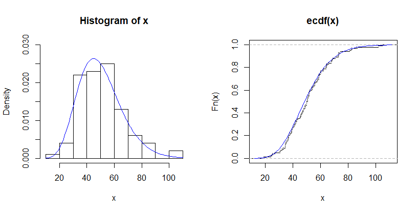
For a small dataset from a gamma distribution, we begin by showing a histogram of the data along with the true density function (left) and an ECDF of the data along with the true CDF (right). For illustration, I chose a small sample so that there will be a clear distinction between exact curves (blue) and estimated ones (red).

set.seed(814)
x = rgamma(100, 10, .2)
par(mfrow=c(1,2))
 hist(x, prob=T, ylim=c(0,.03))
  curve(dgamma(x, 10, .2), add=T, col="blue")
 plot(ecdf(x), pch=".")
  curve(pgamma(x, 10, .2), add=T, col="blue")
par(mfrow=c(1,1))

If the true population distribution is not known, its density function can be estimate by a kernel density estimator (KDE). We use the default KDE in R. The output is two vectors: x-values and y-values for plotting. These vectors are summarized below, and the first six entries in each vector are shown.

density(x)

Call:
        density.default(x = x)

Data: x (100 obs.);     Bandwidth 'bw' = 5.494

       x                 y            
 Min.   :  2.599   Min.   :9.031e-06  
 1st Qu.: 32.251   1st Qu.:9.730e-04  
 Median : 61.902   Median :4.177e-03  
 Mean   : 61.902   Mean   :8.423e-03  
 3rd Qu.: 91.554   3rd Qu.:1.602e-02  
 Max.   :121.205   Max.   :2.527e-02  
head(density(x)$x)
[1] 2.599014 2.831120 3.063227 3.295333 3.527439 3.759546
head(density(x)$y)
[1] 9.030655e-06 1.029092e-05 1.171087e-05 1.327874e-05 1.500377e-05 1.701109e-05

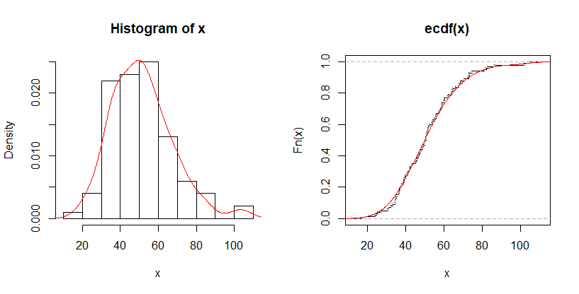
The points in the y-vector are scaled so that the curve enclosed by the KDE will be (almost exactly) 1. The KDE vectors can be used to estimate the CDF. Plotting points are x.k = ecdf(x)$x a and y.k = cumsum(ecdf(x)$y)/sum(ecdf(x)$y). Here are plots of the histogram of x along with the KDE, and the ECDF along with the CDF as estimated via the KDE.

x.k = density(x)$x
y.k = cumsum(density(x)$y)/sum(density(x)$y)
par(mfrow=c(1,2))
 hist(x, prob=T)
  lines(density(x), col="red")
 plot(ecdf(x), pch=".")
  lines(x.k, y.k, col="red")
par(mfrow=c(1,1))