Corrected the margin.
Source Link
Igor F.
  • 9.7k
  • 1
  • 29
  • 63

Maximizing the margin is not just "rhetoric". It is the essential feature of support vector machines and ensures that the trained classifier has the optimal generalization properties. More precisely, making the margin large maximizes the probability that the classification error on new data will be small. The theory behind it is called the Vapnik-Chervonenkis (VC) Theory.

In your question you consider a soft-margin classifier, but the reasoning is equally valid for hard-margin classifiers, which work only on linearly separable datasets. In that case, all your $\zeta_i$'s would simply turn out $0$, thus minimizing the sum in your objective function. Therefore, for simplicity, I'll reformulate your argument for linearly separable data.

Training a support vector machine amounts to optimizing:

$$\min ~ \lVert w \rVert ^2 \\ \text{s.t.} ~ ~ ~ y_i (w^T x_i + b) \ge 1$$

We want to minimize $\lVert w \rVert ^2$ because that maximizes the margin $\gamma$:

$$\gamma = \frac{1}{\lVert w \rVert ^2}$$$$\gamma = \frac{1}{\lVert w \rVert}$$

The constraints ensure not only that all points from the training set are correctly classified, but also that the margin is maximized. As long as there are points for which $y_i (w^T x_i + b) \lt 1$, the training continues by adjusting $w$ and $b$.

Now, you suggest that we can use different constraints:

$$\min ~ \lVert w \rVert ^2 \\ \text{s.t.} ~ ~ ~ y_i (w^T x_i + b) \ge 0$$

The solution to this problem is trivial: Simply set $w=0$ and $b=0$, and $\lVert w \rVert ^2$ will be zero, too. However, this doesn't give you any information about the class boundary: $w$, being now a null vector, doesn't define any hyperplane at all!

Or, to have a look from a different perspective:

Imagine having performed the training using some different learning algorithm, let's say, the perceptron algorithm. You have found some $w$ and $b$ which result in perfect classification on your training set. In other words, your constraint $y_i (w^T x_i + b) \ge 0$ is satisfied for every $i$. But, is this class boundary realistic?

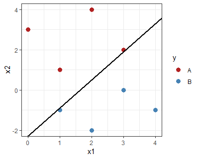
Take the following example: The class boundary separates the blue from the red points, but almost touches one in each class (i.e. the "perceptron" condition is satisfied, but not the SVM condition):

suboptimal separation

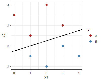
In contrast, the one below has a "large margin", satisfying the SVM condition:

large margin separation

It is intuitively clear that this classifier, having the boundary as far as possible from the training points, has a better chance of good generalization.

Maximizing the margin is not just "rhetoric". It is the essential feature of support vector machines and ensures that the trained classifier has the optimal generalization properties. More precisely, making the margin large maximizes the probability that the classification error on new data will be small. The theory behind it is called the Vapnik-Chervonenkis (VC) Theory.

In your question you consider a soft-margin classifier, but the reasoning is equally valid for hard-margin classifiers, which work only on linearly separable datasets. In that case, all your $\zeta_i$'s would simply turn out $0$, thus minimizing the sum in your objective function. Therefore, for simplicity, I'll reformulate your argument for linearly separable data.

Training a support vector machine amounts to optimizing:

$$\min ~ \lVert w \rVert ^2 \\ \text{s.t.} ~ ~ ~ y_i (w^T x_i + b) \ge 1$$

We want to minimize $\lVert w \rVert ^2$ because that maximizes the margin $\gamma$:

$$\gamma = \frac{1}{\lVert w \rVert ^2}$$

The constraints ensure not only that all points from the training set are correctly classified, but also that the margin is maximized. As long as there are points for which $y_i (w^T x_i + b) \lt 1$, the training continues by adjusting $w$ and $b$.

Now, you suggest that we can use different constraints:

$$\min ~ \lVert w \rVert ^2 \\ \text{s.t.} ~ ~ ~ y_i (w^T x_i + b) \ge 0$$

The solution to this problem is trivial: Simply set $w=0$ and $b=0$, and $\lVert w \rVert ^2$ will be zero, too. However, this doesn't give you any information about the class boundary: $w$, being now a null vector, doesn't define any hyperplane at all!

Or, to have a look from a different perspective:

Imagine having performed the training using some different learning algorithm, let's say, the perceptron algorithm. You have found some $w$ and $b$ which result in perfect classification on your training set. In other words, your constraint $y_i (w^T x_i + b) \ge 0$ is satisfied for every $i$. But, is this class boundary realistic?

Take the following example: The class boundary separates the blue from the red points, but almost touches one in each class (i.e. the "perceptron" condition is satisfied, but not the SVM condition):

suboptimal separation

In contrast, the one below has a "large margin", satisfying the SVM condition:

large margin separation

It is intuitively clear that this classifier, having the boundary as far as possible from the training points, has a better chance of good generalization.
Maximizing the margin is not just "rhetoric". It is the essential feature of support vector machines and ensures that the trained classifier has the optimal generalization properties. More precisely, making the margin large maximizes the probability that the classification error on new data will be small. The theory behind it is called the Vapnik-Chervonenkis (VC) Theory.

In your question you consider a soft-margin classifier, but the reasoning is equally valid for hard-margin classifiers, which work only on linearly separable datasets. In that case, all your $\zeta_i$'s would simply turn out $0$, thus minimizing the sum in your objective function. Therefore, for simplicity, I'll reformulate your argument for linearly separable data.

Training a support vector machine amounts to optimizing:

$$\min ~ \lVert w \rVert ^2 \\ \text{s.t.} ~ ~ ~ y_i (w^T x_i + b) \ge 1$$

We want to minimize $\lVert w \rVert ^2$ because that maximizes the margin $\gamma$:

$$\gamma = \frac{1}{\lVert w \rVert}$$

The constraints ensure not only that all points from the training set are correctly classified, but also that the margin is maximized. As long as there are points for which $y_i (w^T x_i + b) \lt 1$, the training continues by adjusting $w$ and $b$.

Now, you suggest that we can use different constraints:

$$\min ~ \lVert w \rVert ^2 \\ \text{s.t.} ~ ~ ~ y_i (w^T x_i + b) \ge 0$$

The solution to this problem is trivial: Simply set $w=0$ and $b=0$, and $\lVert w \rVert ^2$ will be zero, too. However, this doesn't give you any information about the class boundary: $w$, being now a null vector, doesn't define any hyperplane at all!

Or, to have a look from a different perspective:

Imagine having performed the training using some different learning algorithm, let's say, the perceptron algorithm. You have found some $w$ and $b$ which result in perfect classification on your training set. In other words, your constraint $y_i (w^T x_i + b) \ge 0$ is satisfied for every $i$. But, is this class boundary realistic?

Take the following example: The class boundary separates the blue from the red points, but almost touches one in each class (i.e. the "perceptron" condition is satisfied, but not the SVM condition):

suboptimal separation

In contrast, the one below has a "large margin", satisfying the SVM condition:

large margin separation

It is intuitively clear that this classifier, having the boundary as far as possible from the training points, has a better chance of good generalization.

Rollback to Revision 1
Source Link
Igor F.
  • 9.7k
  • 1
  • 29
  • 63

Maximizing the margin is not just "rhetoric". It is the essential feature of support vector machines and ensures that the trained classifier has the optimal generalization properties. More precisely, making the margin large maximizes the probability that the classification error on new data will be small. The theory behind it is called the Vapnik-Chervonenkis (VC) Theory.

In your question you consider a soft-margin classifier, but the reasoning is equally valid for hard-margin classifiers, which work only on linearly separable datasets. In that case, all your $\zeta_i$'s would simply turn out $0$, thus minimizing the sum in your objective function. Therefore, for simplicity, I'll reformulate your argument for linearly separable data.

Training a support vector machine amounts to optimizing:

$$\min ~ \dfrac{1}{2} \lVert w \rVert ^2 \\ \text{s.t.} ~ ~ ~ y_i (w^T x_i + b) \ge 1$$$$\min ~ \lVert w \rVert ^2 \\ \text{s.t.} ~ ~ ~ y_i (w^T x_i + b) \ge 1$$

We want to minimize $\dfrac{1}{2}\lVert w \rVert ^2$$\lVert w \rVert ^2$ because that maximizes the margin $\gamma$:

$$\gamma = \frac{2}{\lVert w \rVert ^2}$$$$\gamma = \frac{1}{\lVert w \rVert ^2}$$

The constraints ensure not only that all points from the training set are correctly classified, but also that the margin is maximized. As long as there are points for which $y_i (w^T x_i + b) \lt 1$, the training continues by adjusting $w$ and $b$.

Now, you suggest that we can use different constraints:

$$\min ~ \dfrac{1}{2}\lVert w \rVert ^2 \\ \text{s.t.} ~ ~ ~ y_i (w^T x_i + b) \ge 0$$$$\min ~ \lVert w \rVert ^2 \\ \text{s.t.} ~ ~ ~ y_i (w^T x_i + b) \ge 0$$

The solution to this problem is trivial: Simply set $w=0$ and $b=0$, and $\lVert w \rVert ^2$ will be zero, too. However, this doesn't give you any information about the class boundary: $w$, being now a null vector, doesn't define any hyperplane at all!

Or, to have a look from a different perspective:

Imagine having performed the training using some different learning algorithm, let's say, the perceptron algorithm. You have found some $w$ and $b$ which result in perfect classification on your training set. In other words, your constraint $y_i (w^T x_i + b) \ge 0$ is satisfied for every $i$. But, is this class boundary realistic?

Take the following example: The class boundary separates the blue from the red points, but almost touches one in each class (i.e. the "perceptron" condition is satisfied, but not the SVM condition):

suboptimal separation

In contrast, the one below has a "large margin", satisfying the SVM condition:

large margin separation

It is intuitively clear that this classifier, having the boundary as far as possible from the training points, has a better chance of good generalization.

Maximizing the margin is not just "rhetoric". It is the essential feature of support vector machines and ensures that the trained classifier has the optimal generalization properties. More precisely, making the margin large maximizes the probability that the classification error on new data will be small. The theory behind it is called the Vapnik-Chervonenkis (VC) Theory.

In your question you consider a soft-margin classifier, but the reasoning is equally valid for hard-margin classifiers, which work only on linearly separable datasets. In that case, all your $\zeta_i$'s would simply turn out $0$, thus minimizing the sum in your objective function. Therefore, for simplicity, I'll reformulate your argument for linearly separable data.

Training a support vector machine amounts to optimizing:

$$\min ~ \dfrac{1}{2} \lVert w \rVert ^2 \\ \text{s.t.} ~ ~ ~ y_i (w^T x_i + b) \ge 1$$

We want to minimize $\dfrac{1}{2}\lVert w \rVert ^2$ because that maximizes the margin $\gamma$:

$$\gamma = \frac{2}{\lVert w \rVert ^2}$$

The constraints ensure not only that all points from the training set are correctly classified, but also that the margin is maximized. As long as there are points for which $y_i (w^T x_i + b) \lt 1$, the training continues by adjusting $w$ and $b$.

Now, you suggest that we can use different constraints:

$$\min ~ \dfrac{1}{2}\lVert w \rVert ^2 \\ \text{s.t.} ~ ~ ~ y_i (w^T x_i + b) \ge 0$$

The solution to this problem is trivial: Simply set $w=0$ and $b=0$, and $\lVert w \rVert ^2$ will be zero, too. However, this doesn't give you any information about the class boundary: $w$, being now a null vector, doesn't define any hyperplane at all!

Or, to have a look from a different perspective:

Imagine having performed the training using some different learning algorithm, let's say, the perceptron algorithm. You have found some $w$ and $b$ which result in perfect classification on your training set. In other words, your constraint $y_i (w^T x_i + b) \ge 0$ is satisfied for every $i$. But, is this class boundary realistic?

Take the following example: The class boundary separates the blue from the red points, but almost touches one in each class (i.e. the "perceptron" condition is satisfied, but not the SVM condition):

suboptimal separation

In contrast, the one below has a "large margin", satisfying the SVM condition:

large margin separation

It is intuitively clear that this classifier, having the boundary as far as possible from the training points, has a better chance of good generalization.

Maximizing the margin is not just "rhetoric". It is the essential feature of support vector machines and ensures that the trained classifier has the optimal generalization properties. More precisely, making the margin large maximizes the probability that the classification error on new data will be small. The theory behind it is called the Vapnik-Chervonenkis (VC) Theory.

In your question you consider a soft-margin classifier, but the reasoning is equally valid for hard-margin classifiers, which work only on linearly separable datasets. In that case, all your $\zeta_i$'s would simply turn out $0$, thus minimizing the sum in your objective function. Therefore, for simplicity, I'll reformulate your argument for linearly separable data.

Training a support vector machine amounts to optimizing:

$$\min ~ \lVert w \rVert ^2 \\ \text{s.t.} ~ ~ ~ y_i (w^T x_i + b) \ge 1$$

We want to minimize $\lVert w \rVert ^2$ because that maximizes the margin $\gamma$:

$$\gamma = \frac{1}{\lVert w \rVert ^2}$$

The constraints ensure not only that all points from the training set are correctly classified, but also that the margin is maximized. As long as there are points for which $y_i (w^T x_i + b) \lt 1$, the training continues by adjusting $w$ and $b$.

Now, you suggest that we can use different constraints:

$$\min ~ \lVert w \rVert ^2 \\ \text{s.t.} ~ ~ ~ y_i (w^T x_i + b) \ge 0$$

The solution to this problem is trivial: Simply set $w=0$ and $b=0$, and $\lVert w \rVert ^2$ will be zero, too. However, this doesn't give you any information about the class boundary: $w$, being now a null vector, doesn't define any hyperplane at all!

Or, to have a look from a different perspective:

Imagine having performed the training using some different learning algorithm, let's say, the perceptron algorithm. You have found some $w$ and $b$ which result in perfect classification on your training set. In other words, your constraint $y_i (w^T x_i + b) \ge 0$ is satisfied for every $i$. But, is this class boundary realistic?

Take the following example: The class boundary separates the blue from the red points, but almost touches one in each class (i.e. the "perceptron" condition is satisfied, but not the SVM condition):

suboptimal separation

In contrast, the one below has a "large margin", satisfying the SVM condition:

large margin separation

It is intuitively clear that this classifier, having the boundary as far as possible from the training points, has a better chance of good generalization.

fixed objective function, I corrected the margin.
Source Link

Maximizing the margin is not just "rhetoric". It is the essential feature of support vector machines and ensures that the trained classifier has the optimal generalization properties. More precisely, making the margin large maximizes the probability that the classification error on new data will be small. The theory behind it is called the Vapnik-Chervonenkis (VC) Theory.

In your question you consider a soft-margin classifier, but the reasoning is equally valid for hard-margin classifiers, which work only on linearly separable datasets. In that case, all your $\zeta_i$'s would simply turn out $0$, thus minimizing the sum in your objective function. Therefore, for simplicity, I'll reformulate your argument for linearly separable data.

Training a support vector machine amounts to optimizing:

$$\min ~ \lVert w \rVert ^2 \\ \text{s.t.} ~ ~ ~ y_i (w^T x_i + b) \ge 1$$$$\min ~ \dfrac{1}{2} \lVert w \rVert ^2 \\ \text{s.t.} ~ ~ ~ y_i (w^T x_i + b) \ge 1$$

We want to minimize $\lVert w \rVert ^2$$\dfrac{1}{2}\lVert w \rVert ^2$ because that maximizes the margin $\gamma$:

$$\gamma = \frac{1}{\lVert w \rVert ^2}$$$$\gamma = \frac{2}{\lVert w \rVert ^2}$$

The constraints ensure not only that all points from the training set are correctly classified, but also that the margin is maximized. As long as there are points for which $y_i (w^T x_i + b) \lt 1$, the training continues by adjusting $w$ and $b$.

Now, you suggest that we can use different constraints:

$$\min ~ \lVert w \rVert ^2 \\ \text{s.t.} ~ ~ ~ y_i (w^T x_i + b) \ge 0$$$$\min ~ \dfrac{1}{2}\lVert w \rVert ^2 \\ \text{s.t.} ~ ~ ~ y_i (w^T x_i + b) \ge 0$$

The solution to this problem is trivial: Simply set $w=0$ and $b=0$, and $\lVert w \rVert ^2$ will be zero, too. However, this doesn't give you any information about the class boundary: $w$, being now a null vector, doesn't define any hyperplane at all!

Or, to have a look from a different perspective:

Imagine having performed the training using some different learning algorithm, let's say, the perceptron algorithm. You have found some $w$ and $b$ which result in perfect classification on your training set. In other words, your constraint $y_i (w^T x_i + b) \ge 0$ is satisfied for every $i$. But, is this class boundary realistic?

Take the following example: The class boundary separates the blue from the red points, but almost touches one in each class (i.e. the "perceptron" condition is satisfied, but not the SVM condition):

suboptimal separation

In contrast, the one below has a "large margin", satisfying the SVM condition:

large margin separation

It is intuitively clear that this classifier, having the boundary as far as possible from the training points, has a better chance of good generalization.

Maximizing the margin is not just "rhetoric". It is the essential feature of support vector machines and ensures that the trained classifier has the optimal generalization properties. More precisely, making the margin large maximizes the probability that the classification error on new data will be small. The theory behind it is called the Vapnik-Chervonenkis (VC) Theory.

In your question you consider a soft-margin classifier, but the reasoning is equally valid for hard-margin classifiers, which work only on linearly separable datasets. In that case, all your $\zeta_i$'s would simply turn out $0$, thus minimizing the sum in your objective function. Therefore, for simplicity, I'll reformulate your argument for linearly separable data.

Training a support vector machine amounts to optimizing:

$$\min ~ \lVert w \rVert ^2 \\ \text{s.t.} ~ ~ ~ y_i (w^T x_i + b) \ge 1$$

We want to minimize $\lVert w \rVert ^2$ because that maximizes the margin $\gamma$:

$$\gamma = \frac{1}{\lVert w \rVert ^2}$$

The constraints ensure not only that all points from the training set are correctly classified, but also that the margin is maximized. As long as there are points for which $y_i (w^T x_i + b) \lt 1$, the training continues by adjusting $w$ and $b$.

Now, you suggest that we can use different constraints:

$$\min ~ \lVert w \rVert ^2 \\ \text{s.t.} ~ ~ ~ y_i (w^T x_i + b) \ge 0$$

The solution to this problem is trivial: Simply set $w=0$ and $b=0$, and $\lVert w \rVert ^2$ will be zero, too. However, this doesn't give you any information about the class boundary: $w$, being now a null vector, doesn't define any hyperplane at all!

Or, to have a look from a different perspective:

Imagine having performed the training using some different learning algorithm, let's say, the perceptron algorithm. You have found some $w$ and $b$ which result in perfect classification on your training set. In other words, your constraint $y_i (w^T x_i + b) \ge 0$ is satisfied for every $i$. But, is this class boundary realistic?

Take the following example: The class boundary separates the blue from the red points, but almost touches one in each class (i.e. the "perceptron" condition is satisfied, but not the SVM condition):

suboptimal separation

In contrast, the one below has a "large margin", satisfying the SVM condition:

large margin separation

It is intuitively clear that this classifier, having the boundary as far as possible from the training points, has a better chance of good generalization.

Maximizing the margin is not just "rhetoric". It is the essential feature of support vector machines and ensures that the trained classifier has the optimal generalization properties. More precisely, making the margin large maximizes the probability that the classification error on new data will be small. The theory behind it is called the Vapnik-Chervonenkis (VC) Theory.

In your question you consider a soft-margin classifier, but the reasoning is equally valid for hard-margin classifiers, which work only on linearly separable datasets. In that case, all your $\zeta_i$'s would simply turn out $0$, thus minimizing the sum in your objective function. Therefore, for simplicity, I'll reformulate your argument for linearly separable data.

Training a support vector machine amounts to optimizing:

$$\min ~ \dfrac{1}{2} \lVert w \rVert ^2 \\ \text{s.t.} ~ ~ ~ y_i (w^T x_i + b) \ge 1$$

We want to minimize $\dfrac{1}{2}\lVert w \rVert ^2$ because that maximizes the margin $\gamma$:

$$\gamma = \frac{2}{\lVert w \rVert ^2}$$

The constraints ensure not only that all points from the training set are correctly classified, but also that the margin is maximized. As long as there are points for which $y_i (w^T x_i + b) \lt 1$, the training continues by adjusting $w$ and $b$.

Now, you suggest that we can use different constraints:

$$\min ~ \dfrac{1}{2}\lVert w \rVert ^2 \\ \text{s.t.} ~ ~ ~ y_i (w^T x_i + b) \ge 0$$

The solution to this problem is trivial: Simply set $w=0$ and $b=0$, and $\lVert w \rVert ^2$ will be zero, too. However, this doesn't give you any information about the class boundary: $w$, being now a null vector, doesn't define any hyperplane at all!

Or, to have a look from a different perspective:

Imagine having performed the training using some different learning algorithm, let's say, the perceptron algorithm. You have found some $w$ and $b$ which result in perfect classification on your training set. In other words, your constraint $y_i (w^T x_i + b) \ge 0$ is satisfied for every $i$. But, is this class boundary realistic?

Take the following example: The class boundary separates the blue from the red points, but almost touches one in each class (i.e. the "perceptron" condition is satisfied, but not the SVM condition):

suboptimal separation

In contrast, the one below has a "large margin", satisfying the SVM condition:

large margin separation

It is intuitively clear that this classifier, having the boundary as far as possible from the training points, has a better chance of good generalization.

Bounty Ended with 50 reputation awarded by Cagdas Ozgenc
Source Link
Igor F.
  • 9.7k
  • 1
  • 29
  • 63
Loading