added 16 characters in body
Source Link
BruceET
  • 57.6k
  • 2
  • 36
  • 94

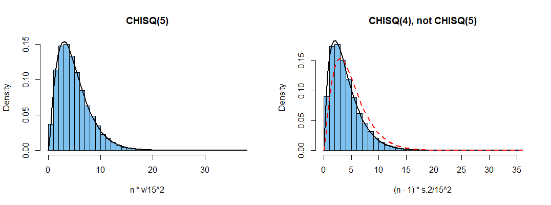
If you have data $X_1, X_2, \dots, X_n$ randomly sampled from $\mathsf{Norm}(\mu, \sigma),$ with $\mu$ known and $\sigma$ unknown, then $V = \frac{1}{n}\sum_{i=1}^n (X_i - \mu)^2$ has $E(V) = \sigma^2,$ with $\frac{nV}{\sigma} \sim \mathsf{Chisq}(\nu = n).$ The proof follows directly from the definition of $\mathsf{Chisq}(\nu = n)$ as the distribution of the sum of $n$ independent standard normal random variables.

However if $\mu$ is also unknown, then $S^2 = \frac{1}{n-1}\sum_{i=1}^n (X_i - \bar X)^2,$ where $\mu$ is estimated by $\bar X = \frac{1}{n} X_i,$ is the usual unbiased estimator of $\sigma^2,$ with $E(S^2) = \sigma^2$ and $\frac{(n-1)S^2}{\sigma^2} \sim \mathsf{Chisq}(\nu = n-1).$ Informally, people may say that one degree of freedom is 'lost' in the estimatiion of $\mu.$ However, a formal proof requires moment generating functions or a transformation of an $n$-variate normal distribution.

In the latter case ($\mu$ unknown), some statisticians have argued that it is better to use $Q = \frac{n-1}{n}S^2$ $= \frac{1}{n}\sum_{i=1}^n (X_i - \bar X)^2$ because, for normal data, it has a smaller mean squared error than $S^2.$ It is true that $\mathrm{MSE}(Q) < \mathrm{MSE}(S^2),$ but it is not obvious that minimizing MSE is a suitable criterion for choosing the best estimator. [And if minimizing MSE is to be the criterion, then $Q^\prime=\frac{n-1}{n+1}S^2$ has even smaller MSE, and both variants are biased.]

Simulations and some graphs:

set.seed(626)
m = 10^5;  n = 5
x = rnorm(m*n, 100, 15)
DTA = matrix(x, nrow=m)
v = rowSums((DTA-100)^2)/n
s.2 = apply(DTA, 1, var)
par(mfrow=c(1,2))
 hdr="CHISQ(5)"
 hist(n*v/15^2, prob=T, br=40, col="skyblue2", main=hdr)
  curve(dchisq(x,5), add=T, lwd=2)
 hdr="CHISQ(4), not CHISQ(5)"
 hist((n-1)*s.2/15^2, prob=T, br=40, col="skyblue2", main=hdr)
  curve(dchisq(x,4), add=T, lwd=2)
  curve(dchisq(x,5), add=T, col="red", lty="dashed", lwd=2)
par(mfrow=c(1,1))

enter image description here

mean((s.2 - 15)^2)
[1] 69444.44       # aprx. MSE S^2
q = (n-1)*s.2/n
mean((q - 15)^2)   
[1] 43445.15       # aprx. MSE Q
q1 =(n-1)*s.2/(n+1)
mean((q1 - 15)^2)
[1] 29488.79       # even smaller MSE

enter image description here

It seems that MSE is very heavily influenced by the right tail. Too heavily?

par(mfrow=c(1,3))
 hist(s.2, prob=T, xlim=c(0,max(s.2)), col="skyblue2")
  abline(v=15^2, col="red")
 hist(q, prob=T, xlim=c(0,max(s.2)), col="skyblue2")
  abline(v=15^2, col="red")
 hist(q1, prob=T, xlim=c(0,max(s.2)), col="skyblue2")
  abline(v=15^2, col="red")
par(mfrow=c(1,1))

If you have data $X_1, X_2, \dots, X_n$ randomly sampled from $\mathsf{Norm}(\mu, \sigma),$ with $\mu$ known and $\sigma$ unknown, then $V = \frac{1}{n}\sum_{i=1}^n (X_i - \mu)^2$ has $E(V) = \sigma^2,$ with $\frac{nV}{\sigma} \sim \mathsf{Chisq}(\nu = n).$ The proof follows directly from the definition of $\mathsf{Chisq}(\nu = n)$ as the distribution of the sum of $n$ independent standard normal random variables.

However if $\mu$ is also unknown, then $S^2 = \frac{1}{n-1}\sum_{i=1}^n (X_i - \bar X)^2,$ where $\mu$ is estimated by $\bar X = \frac{1}{n} X_i,$ is the usual unbiased estimator of $\sigma^2,$ with $E(S^2) = \sigma^2$ and $\frac{(n-1)S^2}{\sigma^2} \sim \mathsf{Chisq}(\nu = n-1).$ Informally, people may say that one degree of freedom is 'lost' in the estimatiion of $\mu.$ However, a formal proof requires moment generating functions or a transformation of an $n$-variate normal distribution.

In the latter case, some statisticians have argued that it is better to use $Q = \frac{n-1}{n}S^2$ $= \frac{1}{n}\sum_{i=1}^n (X_i - \bar X)^2$ because, for normal data, it has a smaller mean squared error than $S^2.$ It is true that $\mathrm{MSE}(Q) < \mathrm{MSE}(S^2),$ but it is not obvious that minimizing MSE is a suitable criterion for choosing the best estimator. [And if minimizing MSE is to be the criterion, then $Q^\prime=\frac{n-1}{n+1}S^2$ has even smaller MSE, and both variants are biased.]

Simulations and some graphs:

set.seed(626)
m = 10^5;  n = 5
x = rnorm(m*n, 100, 15)
DTA = matrix(x, nrow=m)
v = rowSums((DTA-100)^2)/n
s.2 = apply(DTA, 1, var)
par(mfrow=c(1,2))
 hdr="CHISQ(5)"
 hist(n*v/15^2, prob=T, br=40, col="skyblue2", main=hdr)
  curve(dchisq(x,5), add=T, lwd=2)
 hdr="CHISQ(4), not CHISQ(5)"
 hist((n-1)*s.2/15^2, prob=T, br=40, col="skyblue2", main=hdr)
  curve(dchisq(x,4), add=T, lwd=2)
  curve(dchisq(x,5), add=T, col="red", lty="dashed", lwd=2)
par(mfrow=c(1,1))

enter image description here

mean((s.2 - 15)^2)
[1] 69444.44       # aprx. MSE S^2
q = (n-1)*s.2/n
mean((q - 15)^2)   
[1] 43445.15       # aprx. MSE Q
q1 =(n-1)*s.2/(n+1)
mean((q1 - 15)^2)
[1] 29488.79       # even smaller MSE

enter image description here

par(mfrow=c(1,3))
 hist(s.2, prob=T, xlim=c(0,max(s.2)), col="skyblue2")
  abline(v=15^2, col="red")
 hist(q, prob=T, xlim=c(0,max(s.2)), col="skyblue2")
  abline(v=15^2, col="red")
 hist(q1, prob=T, xlim=c(0,max(s.2)), col="skyblue2")
  abline(v=15^2, col="red")
par(mfrow=c(1,1))
If you have data $X_1, X_2, \dots, X_n$ randomly sampled from $\mathsf{Norm}(\mu, \sigma),$ with $\mu$ known and $\sigma$ unknown, then $V = \frac{1}{n}\sum_{i=1}^n (X_i - \mu)^2$ has $E(V) = \sigma^2,$ with $\frac{nV}{\sigma} \sim \mathsf{Chisq}(\nu = n).$ The proof follows directly from the definition of $\mathsf{Chisq}(\nu = n)$ as the distribution of the sum of $n$ independent standard normal random variables.

However if $\mu$ is also unknown, then $S^2 = \frac{1}{n-1}\sum_{i=1}^n (X_i - \bar X)^2,$ where $\mu$ is estimated by $\bar X = \frac{1}{n} X_i,$ is the usual unbiased estimator of $\sigma^2,$ with $E(S^2) = \sigma^2$ and $\frac{(n-1)S^2}{\sigma^2} \sim \mathsf{Chisq}(\nu = n-1).$ Informally, people may say that one degree of freedom is 'lost' in the estimatiion of $\mu.$ However, a formal proof requires moment generating functions or a transformation of an $n$-variate normal distribution.

In the latter case ($\mu$ unknown), some statisticians have argued that it is better to use $Q = \frac{n-1}{n}S^2$ $= \frac{1}{n}\sum_{i=1}^n (X_i - \bar X)^2$ because, for normal data, it has a smaller mean squared error than $S^2.$ It is true that $\mathrm{MSE}(Q) < \mathrm{MSE}(S^2),$ but it is not obvious that minimizing MSE is a suitable criterion for choosing the best estimator. [And if minimizing MSE is to be the criterion, then $Q^\prime=\frac{n-1}{n+1}S^2$ has even smaller MSE, and both variants are biased.]

Simulations and some graphs:

set.seed(626)
m = 10^5;  n = 5
x = rnorm(m*n, 100, 15)
DTA = matrix(x, nrow=m)
v = rowSums((DTA-100)^2)/n
s.2 = apply(DTA, 1, var)
par(mfrow=c(1,2))
 hdr="CHISQ(5)"
 hist(n*v/15^2, prob=T, br=40, col="skyblue2", main=hdr)
  curve(dchisq(x,5), add=T, lwd=2)
 hdr="CHISQ(4), not CHISQ(5)"
 hist((n-1)*s.2/15^2, prob=T, br=40, col="skyblue2", main=hdr)
  curve(dchisq(x,4), add=T, lwd=2)
  curve(dchisq(x,5), add=T, col="red", lty="dashed", lwd=2)
par(mfrow=c(1,1))

enter image description here

mean((s.2 - 15)^2)
[1] 69444.44       # aprx. MSE S^2
q = (n-1)*s.2/n
mean((q - 15)^2)   
[1] 43445.15       # aprx. MSE Q
q1 =(n-1)*s.2/(n+1)
mean((q1 - 15)^2)
[1] 29488.79       # even smaller MSE

enter image description here

It seems that MSE is very heavily influenced by the right tail. Too heavily?

par(mfrow=c(1,3))
 hist(s.2, prob=T, xlim=c(0,max(s.2)), col="skyblue2")
  abline(v=15^2, col="red")
 hist(q, prob=T, xlim=c(0,max(s.2)), col="skyblue2")
  abline(v=15^2, col="red")
 hist(q1, prob=T, xlim=c(0,max(s.2)), col="skyblue2")
  abline(v=15^2, col="red")
par(mfrow=c(1,1))
Source Link
BruceET
  • 57.6k
  • 2
  • 36
  • 94

If you have data $X_1, X_2, \dots, X_n$ randomly sampled from $\mathsf{Norm}(\mu, \sigma),$ with $\mu$ known and $\sigma$ unknown, then $V = \frac{1}{n}\sum_{i=1}^n (X_i - \mu)^2$ has $E(V) = \sigma^2,$ with $\frac{nV}{\sigma} \sim \mathsf{Chisq}(\nu = n).$ The proof follows directly from the definition of $\mathsf{Chisq}(\nu = n)$ as the distribution of the sum of $n$ independent standard normal random variables.

However if $\mu$ is also unknown, then $S^2 = \frac{1}{n-1}\sum_{i=1}^n (X_i - \bar X)^2,$ where $\mu$ is estimated by $\bar X = \frac{1}{n} X_i,$ is the usual unbiased estimator of $\sigma^2,$ with $E(S^2) = \sigma^2$ and $\frac{(n-1)S^2}{\sigma^2} \sim \mathsf{Chisq}(\nu = n-1).$ Informally, people may say that one degree of freedom is 'lost' in the estimatiion of $\mu.$ However, a formal proof requires moment generating functions or a transformation of an $n$-variate normal distribution.

In the latter case, some statisticians have argued that it is better to use $Q = \frac{n-1}{n}S^2$ $= \frac{1}{n}\sum_{i=1}^n (X_i - \bar X)^2$ because, for normal data, it has a smaller mean squared error than $S^2.$ It is true that $\mathrm{MSE}(Q) < \mathrm{MSE}(S^2),$ but it is not obvious that minimizing MSE is a suitable criterion for choosing the best estimator. [And if minimizing MSE is to be the criterion, then $Q^\prime=\frac{n-1}{n+1}S^2$ has even smaller MSE, and both variants are biased.]

Simulations and some graphs:

set.seed(626)
m = 10^5;  n = 5
x = rnorm(m*n, 100, 15)
DTA = matrix(x, nrow=m)
v = rowSums((DTA-100)^2)/n
s.2 = apply(DTA, 1, var)
par(mfrow=c(1,2))
 hdr="CHISQ(5)"
 hist(n*v/15^2, prob=T, br=40, col="skyblue2", main=hdr)
  curve(dchisq(x,5), add=T, lwd=2)
 hdr="CHISQ(4), not CHISQ(5)"
 hist((n-1)*s.2/15^2, prob=T, br=40, col="skyblue2", main=hdr)
  curve(dchisq(x,4), add=T, lwd=2)
  curve(dchisq(x,5), add=T, col="red", lty="dashed", lwd=2)
par(mfrow=c(1,1))

enter image description here

mean((s.2 - 15)^2)
[1] 69444.44       # aprx. MSE S^2
q = (n-1)*s.2/n
mean((q - 15)^2)   
[1] 43445.15       # aprx. MSE Q
q1 =(n-1)*s.2/(n+1)
mean((q1 - 15)^2)
[1] 29488.79       # even smaller MSE

enter image description here

par(mfrow=c(1,3))
 hist(s.2, prob=T, xlim=c(0,max(s.2)), col="skyblue2")
  abline(v=15^2, col="red")
 hist(q, prob=T, xlim=c(0,max(s.2)), col="skyblue2")
  abline(v=15^2, col="red")
 hist(q1, prob=T, xlim=c(0,max(s.2)), col="skyblue2")
  abline(v=15^2, col="red")
par(mfrow=c(1,1))