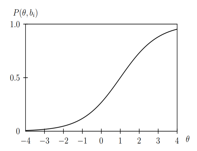
The 1PL (one-parameter logistic model) is given by
$$p(\theta|b_i) = \dfrac{\exp(\theta - b_i)}{1 +\exp(\theta - b_i)}.$$
This is trying to model the probability of solving a given item with difficulty $b_i$ when the person has the ability $\theta$. It is clear that larger $\theta$ will increase the probability of solving the task if the difficulty $b_i$ does not change. Increasing $b_i$ will decrease the probability of solving a task if the ability $\theta$ is fixed.
This function has a shape like the letter s if $\theta$ is treated as the independent variable and the probability is your dependent variable. This is the reason why this function is of a sigmoid-type (sigma: greek letter for s).
The 2PL (two-parameter logistic model) is given by
$$p(\theta|a_i, b_i) = \dfrac{\exp[a_i(\theta - b_i)]}{1 +\exp[a_i(\theta - b_i)]}.$$
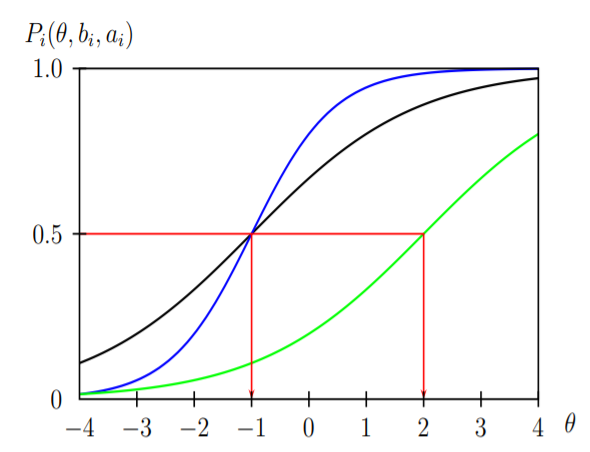
The effect $a_i$ (discrimination factor) is that the transition from the lower probabilities to larger probabilities will be more rapid. The following picture contains a black and a blue function. Both functions have the same difficulty $b_i$ but the discrimination $a_i$ is different. The discrimination of the blue function is larger than the discrimination of the black function.
Items with large discrimination are very good for distinguishing between people with abilities larger than the item difficulty and people with abilities smaller than the item difficulty. But these items are very by for discriminating abilities farther away from the difficulty of the item. See the next paragraph for an item with ideal discrimination ($a_i \to \infty$).
For the limit $a_i \to \infty$ we will obtain a step function. It will be zero on the left-hand side and 1 on the right-hand side of the ability $\theta$ which corresponds to the difficulty of the item. This model is called the deterministic Guttman-Model. It is clear that you will not be able to distinguish abilities larger than the difficulty (curve is flat).
Credit for pictures: Both pictures were taken from this source.


