Commonmark migration
Source Link

You can use the method of moments as neatly set out for you in the [Wikipedia article on the beta distribution][1]Wikipedia article on the beta distribution. Here is some code to get you started:

![enter image description here][2]enter image description here

From here you can use Bayesian techniques to confront your prior distribution with the likelihood of the actual data, and hence produce a posterior distribution that combines the two. [1]: http://en.wikipedia.org/wiki/Beta_distribution#Two_unknown_parameters [2]: https://i.sstatic.net/61Otd.png
You can use the method of moments as neatly set out for you in the [Wikipedia article on the beta distribution][1]. Here is some code to get you started:

![enter image description here][2]

From here you can use Bayesian techniques to confront your prior distribution with the likelihood of the actual data, and hence produce a posterior distribution that combines the two. [1]: http://en.wikipedia.org/wiki/Beta_distribution#Two_unknown_parameters [2]: https://i.sstatic.net/61Otd.png

You can use the method of moments as neatly set out for you in the Wikipedia article on the beta distribution. Here is some code to get you started:

enter image description here

From here you can use Bayesian techniques to confront your prior distribution with the likelihood of the actual data, and hence produce a posterior distribution that combines the two.

corrected fragment of old code (wrong variable name)
Source Link
Peter Ellis
  • 17.8k
  • 1
  • 51
  • 90
u <- with(expert, probs %*% prior)
v <- with(expert, ((probs-M1u)^2) %*% prior)

alpha <- u* (  (u*(1-u)) /v  -1)
beta <- (1-u) * (( u*(1-u))/v-1)

x <- 0:1000/1000

png("beta and point estimates.png", 400,400, res=72)
    plot(x, dbeta(x, alpha, beta), type="l", bty="l", ylim=c(0,3), 
        ylab="Density", xlab="Probability",
        main="Original expert point estimates,\nand beta distribution")
    with(expert, points(probs, prior/sum(.1 * prior)prior*10))
dev.off()
u <- with(expert, probs %*% prior)
v <- with(expert, ((probs-M1)^2) %*% prior)

alpha <- u* (  (u*(1-u)) /v  -1)
beta <- (1-u) * (( u*(1-u))/v-1)

x <- 0:1000/1000

png("beta and point estimates.png", 400,400, res=72)
    plot(x, dbeta(x, alpha, beta), type="l", bty="l", ylim=c(0,3), 
        ylab="Density", xlab="Probability",
        main="Original expert point estimates,\nand beta distribution")
    with(expert, points(probs, prior/sum(.1 * prior)))
dev.off()
u <- with(expert, probs %*% prior)
v <- with(expert, ((probs-u)^2) %*% prior)

alpha <- u* (  (u*(1-u)) /v  -1)
beta <- (1-u) * (( u*(1-u))/v-1)

x <- 0:1000/1000

png("beta and point estimates.png", 400,400, res=72)
    plot(x, dbeta(x, alpha, beta), type="l", bty="l", ylim=c(0,3), 
        ylab="Density", xlab="Probability",
        main="Original expert point estimates,\nand beta distribution")
    with(expert, points(probs, prior*10))
dev.off()
Source Link
Peter Ellis
  • 17.8k
  • 1
  • 51
  • 90

To expand on @Glen_b's answer. A beta distribution is the standard answer here, although it should be noted that it is possible (and also not uncommon) to not try to smooth/model the prior distribution at all but just use some raw point estimates... putting that aside, let us say you think the probability of an occurance can be anywhere between 0 and 1 but you have an expert guess of the chance of that probability being correct for each of 0.1, 0.2, etc. That is, your expert (perhaps you) thinks the chance that that probability is 0.1 is only 0.01; the chance it really is 0.2 is 0.015, and so on.

You can use the method of moments as neatly set out for you in the [Wikipedia article on the beta distribution][1]. Here is some code to get you started:

expert <- data.frame(
    probs=1:9/10, 
    prior=c(.01,.15,.3,.2,.14, .1,.05,.04,.01)
)

sum(expert$prior) # check equal to 1

That is, the prior estimates of the chance of each probability are:

> expert
  probs prior
1   0.1  0.01
2   0.2  0.15
3   0.3  0.30
4   0.4  0.20
5   0.5  0.14
6   0.6  0.10
7   0.7  0.05
8   0.8  0.04
9   0.9  0.01

So now to use the method of moments to turn this into a beta distribution that can summarise it:

u <- with(expert, probs %*% prior)
v <- with(expert, ((probs-M1)^2) %*% prior)

alpha <- u* (  (u*(1-u)) /v  -1)
beta <- (1-u) * (( u*(1-u))/v-1)

x <- 0:1000/1000

png("beta and point estimates.png", 400,400, res=72)
    plot(x, dbeta(x, alpha, beta), type="l", bty="l", ylim=c(0,3), 
        ylab="Density", xlab="Probability",
        main="Original expert point estimates,\nand beta distribution")
    with(expert, points(probs, prior/sum(.1 * prior)))
dev.off()

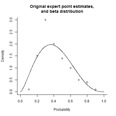
You can see from the image below that the beta distribution is an ok summary of the expert's opinion but it isn't quite the same - basically, the expert's view on the chance of 0.3 being the true probability are a bit of a spike in their prior distribution.

![enter image description here][2]

From here you can use Bayesian techniques to confront your prior distribution with the likelihood of the actual data, and hence produce a posterior distribution that combines the two. [1]: http://en.wikipedia.org/wiki/Beta_distribution#Two_unknown_parameters [2]: https://i.sstatic.net/61Otd.png