If you use statistical software to test the hypothesis $H_0: \mu_1 \le \mu_2$ against $H_a: \mu_1 > m_2$ you will typically get a 95% confidence interval for $\mu_1 - \mu_2$ as part of the output.

Suppose you have data similar to the fictitious data, simulated using R statistical software below:

set.seed(2022)
x1 = rnorm(1000, 50, 7)
x2 = rnorm(1000, 55, 8)

summary(x1)
  Min. 1st Qu.  Median    Mean 3rd Qu.    Max. 
  25.67   45.28   49.65   50.01   54.79   76.36 
length(x1);  sd(x1)
[1] 1000              # sample size
[1] 6.987677          # sample standard deviation

summary(x2)
   Min. 1st Qu.  Median    Mean 3rd Qu.    Max. 
  25.86   49.61   54.99   54.97   60.66   79.58
length(x2);  sd(x2)
[1] 1000
[1] 8.190649

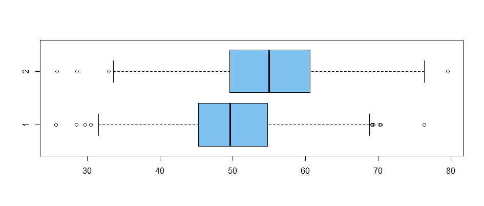
boxplot(x1, x2, horizontal=T, col="skyblue2")

Then a Welch two-sample t test, which does not assume that treatment and control populations have the same variance, goes as shown below. Because the P-value is near $0,$ we reject $H_0$ in favor of the one-sided alternative $H_0.$ The 95% one-sided 95% confidence interval is $(-\infty, -4.40)$ so that $\mu_1 - \mu_2,$ estimated by $\bar X_1 - \bar X_2 = 50.00961 - 54.97116 = -4.96155$ is likely less than the upper bound $-4.40128 \approx -4.40.$

        Welch Two Sample t-test

data:  x1 and x2
t = -14.573, df = 1949.6, p-value < 2.2e-16
alternative hypothesis: true difference in means is less than 0
95 percent confidence interval:
 -Inf -4.40128
sample estimates:
mean of x mean of y 
 50.00961  54.97116 

If you want a 2-sided 95% CI, then you can get it as part of the output for a 2-tailed (or 2-sided) test, specifically $(-5.63, -4.29),$ which is centered at $\bar X_1 - \bar X_2 = 50.00961 - 54.97116 = -4.96155 \approx -4.96.$

t.test(x1,x2)$conf.int
[1] -5.629265 -4.293849
attr(,"conf.level")
[1] 0.95

Output from Minitab statistical software for summarized data above, is shown below, where 0.000 means $< 0.0005:$

Two-Sample T-Test and CI 

Sample     N   Mean  StDev  SE Mean
1       1000  50.01   6.99     0.22
2       1000  54.97   8.19     0.26

Difference = μ (1) - μ (2)
Estimate for difference:  -4.960
95% upper bound for difference:  -4.400
T-Test of difference = 0 (vs <): 
 T-Value = -14.57  P-Value = 0.000  DF = 1949

Again here, the two-sided 95% CI $(-5.628, -4.292)$ accompanies the two-sided test.

$$\bar X_1 - \bar X_2 \pm t^*\sqrt{\frac{S_1^2}{n_1}+\frac{S_2^2}{n_2}}.$$

Two-Sample T-Test and CI 

Sample     N   Mean  StDev  SE Mean
1       1000  50.01   6.99     0.22
2       1000  54.97   8.19     0.26


Difference = μ (1) - μ (2)
Estimate for difference:  -4.960
95% CI for difference:  (-5.628, -4.292)
T-Test of difference = 0 (vs ≠): T-Value = -14.57  P-Value = 0.000  DF = 1949

Both programs use the following formula for the 2-sided 95% confidence interval of $\mu_1-\mu_2:$

$$\bar X_1 - \bar X_2 \pm t^*\sqrt{\frac{S_1^2}{n_1}+\frac{S_2^2}{n_2}},$$ where $n_i, \bar X_i, S^2_i$ are the sample size, mean, and variance, respectively, of the $i$th sample, and $t^*$ cuts probability $0.025$ from the upper tail of Student's t distribution with the appropriate degrees of freedom. In my example $t^*=1.96.$