added 98 characters in body
Source Link
Shawn Hemelstrand
  • 18.4k
  • 6
  • 35
  • 92
#### Simulate Groups ####
set.seed(123)

group.1 <- rnorm(n = 1000,
                 mean = 100000,
                 sd = 10000)

group.2 <- rnorm(n = 1000,
                 mean = 121000120000,
                 sd = 5000)

df <- data.frame(CitiBank = group.1,
                 BOA = group.2)

#### Test Groups ####
t.test(group.2,
       group.1,
       alternative = "greater")
    Welch Two Sample t-test

data:  group.2 and group.1
t = 5956.82298, df = 1484.2, p-value < 2.2e-16
alternative hypothesis: true difference in means is greater than 0
95 percent confidence interval:
 2047119471.87      Inf
sample estimates:
mean of x mean of y 
 121212120212.3  100161.3 

However, if we plot the critical cutoff zones used for a two-tailed test and compare them to a one-tailed test:

enter image description here

#### Plot ####
library(tidyverse)
library(ggpubr)

p1 <- df %>% 
  gather() %>% 
  ggplot(aes(x=value,
             fill=key))+
  geom_density(alpha = .5,
               linewidth = 1)+
  theme_classic()+
  scale_fill_manual(values = c("black","white"))+
  geom_vline(aes(xintercept = mean(group.1)),
             color = "red",
             linetype = "dashed",
             linewidth = 1)+
  geom_vline(aes(xintercept = mean(group.2)),
             color = "red",
             linetype = "dashed",
             linewidth = 1)+
  geom_vline(aes(xintercept = mean(group.1) + 1.96*sd(group.1)),
             color = "blue",
             linetype = "dashed",
             linewidth = 1)+
  geom_vline(aes(xintercept = mean(group.1) - 1.96*sd(group.1)),
             color = "blue",
             linetype = "dashed",
             linewidth = 1)+
  labs(x="Salary",
       y = "Density",
       fill = "Group",
       title = "Salary Comparison with Two-Tailed Test")+
  scale_x_continuous(n.breaks = 10)

p2 <- df %>% 
  gather() %>% 
  ggplot(aes(x=value,
             fill=key))+
  geom_density(alpha = .5,
               linewidth = 1)+
  theme_classic()+
  scale_fill_manual(values = c("black","white"))+
  geom_vline(aes(xintercept = mean(group.1)),
             color = "red",
             linetype = "dashed",
             linewidth = 1)+
  geom_vline(aes(xintercept = mean(group.2)),
             color = "red",
             linetype = "dashed",
             linewidth = 1)+
  geom_vline(aes(xintercept = mean(group.1) + 1.645*sd(group.1)),
             color = "blue",
             linetype = "dashed",
             linewidth = 1)+
  labs(x="Salary",
       y = "Density",
       fill = "Group",
       title = "Salary Comparison with One-Tailed Test")+
  scale_x_continuous(n.breaks = 10)

ggarrange(p1,p2, ncol = 1)

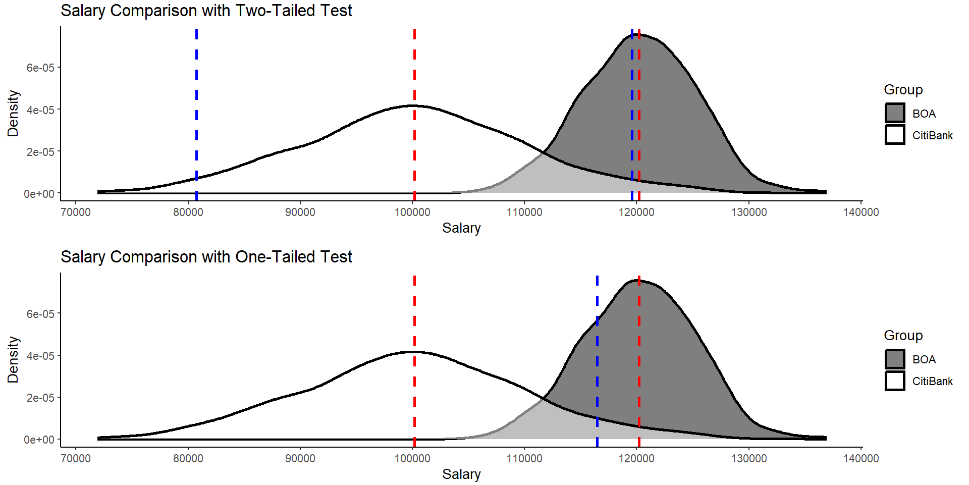
You will notice that we barely made the cutoff if using at two-tailed test (for simplicity, I just used two SD above the mean, but it should be a z-score above or below 1.96 to be precise).get these plots:

enter image description here

The red dashed lines are the means of each group and the blue dashed lines are the critical regions to reject the null. The plot on top shows cutoffs for the two-tailed test whereas the plot on the bottom shows a one-tailed test. You can see that for the two-tailed test we barely pass the cutoff criterion. However, we have far surpassed it in the one-tailed case.

#### Simulate Groups ####
set.seed(123)

group.1 <- rnorm(n = 1000,
                 mean = 100000,
                 sd = 10000)

group.2 <- rnorm(n = 1000,
                 mean = 121000,
                 sd = 5000)

df <- data.frame(CitiBank = group.1,
                 BOA = group.2)

#### Test Groups ####
t.test(group.2,
       group.1,
       alternative = "greater")
Welch Two Sample t-test

data:  group.2 and group.1
t = 59.822, df = 1484.2, p-value < 2.2e-16
alternative hypothesis: true difference in means is greater than 0
95 percent confidence interval:
 20471.87      Inf
sample estimates:
mean of x mean of y 
 121212.3  100161.3 

However, if we plot the critical cutoff zones used for a two-tailed test:

enter image description here

You will notice that we barely made the cutoff if using at two-tailed test (for simplicity, I just used two SD above the mean, but it should be a z-score above or below 1.96 to be precise). The red dashed lines are the means of each group and the blue dashed lines are the critical regions to reject the null.

#### Simulate Groups ####
set.seed(123)

group.1 <- rnorm(n = 1000,
                 mean = 100000,
                 sd = 10000)

group.2 <- rnorm(n = 1000,
                 mean = 120000,
                 sd = 5000)

df <- data.frame(CitiBank = group.1,
                 BOA = group.2)

#### Test Groups ####
t.test(group.2,
       group.1,
       alternative = "greater")
    Welch Two Sample t-test

data:  group.2 and group.1
t = 56.98, df = 1484.2, p-value < 2.2e-16
alternative hypothesis: true difference in means is greater than 0
95 percent confidence interval:
 19471.87      Inf
sample estimates:
mean of x mean of y 
 120212.3  100161.3 

However, if we plot the critical cutoff zones used for a two-tailed test and compare them to a one-tailed test:

#### Plot ####
library(tidyverse)
library(ggpubr)

p1 <- df %>% 
  gather() %>% 
  ggplot(aes(x=value,
             fill=key))+
  geom_density(alpha = .5,
               linewidth = 1)+
  theme_classic()+
  scale_fill_manual(values = c("black","white"))+
  geom_vline(aes(xintercept = mean(group.1)),
             color = "red",
             linetype = "dashed",
             linewidth = 1)+
  geom_vline(aes(xintercept = mean(group.2)),
             color = "red",
             linetype = "dashed",
             linewidth = 1)+
  geom_vline(aes(xintercept = mean(group.1) + 1.96*sd(group.1)),
             color = "blue",
             linetype = "dashed",
             linewidth = 1)+
  geom_vline(aes(xintercept = mean(group.1) - 1.96*sd(group.1)),
             color = "blue",
             linetype = "dashed",
             linewidth = 1)+
  labs(x="Salary",
       y = "Density",
       fill = "Group",
       title = "Salary Comparison with Two-Tailed Test")+
  scale_x_continuous(n.breaks = 10)

p2 <- df %>% 
  gather() %>% 
  ggplot(aes(x=value,
             fill=key))+
  geom_density(alpha = .5,
               linewidth = 1)+
  theme_classic()+
  scale_fill_manual(values = c("black","white"))+
  geom_vline(aes(xintercept = mean(group.1)),
             color = "red",
             linetype = "dashed",
             linewidth = 1)+
  geom_vline(aes(xintercept = mean(group.2)),
             color = "red",
             linetype = "dashed",
             linewidth = 1)+
  geom_vline(aes(xintercept = mean(group.1) + 1.645*sd(group.1)),
             color = "blue",
             linetype = "dashed",
             linewidth = 1)+
  labs(x="Salary",
       y = "Density",
       fill = "Group",
       title = "Salary Comparison with One-Tailed Test")+
  scale_x_continuous(n.breaks = 10)

ggarrange(p1,p2, ncol = 1)

You will get these plots:

enter image description here

The red dashed lines are the means of each group and the blue dashed lines are the critical regions to reject the null. The plot on top shows cutoffs for the two-tailed test whereas the plot on the bottom shows a one-tailed test. You can see that for the two-tailed test we barely pass the cutoff criterion. However, we have far surpassed it in the one-tailed case.
Source Link
Shawn Hemelstrand
  • 18.4k
  • 6
  • 35
  • 92

Some Scenarios

I wanted to focus on one particular part of your question:

I just wanted to see if there are real life, practical applications of the 1 sided test in the real world

Here are some practical examples:

  • "Is my company's starting salary larger than a rival company?"
  • "Do students at my school receive less student aid than other schools?"
  • "Are people from my graduating class taller than other classes before me?"

These are all questions that can be answered by one-sided tests. However, this is also where hypothesis testing is very important. Using the first example, we may have a litany of informal evidence that seems to suggest salaries are greater at another company (feedback from employees there, bigger offices at their company, etc.). Rather than just asking ourselves "are their salaries different from ours?" an easier question to answer may be the one already posed: are they higher? Knowing this information would be super useful if you decided to change companies down the road.

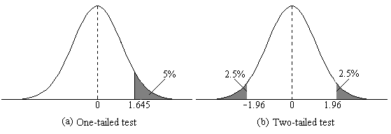
Remember that your chances of rejecting the null hypothesis in one direction increase as a result of how big the tail is compared to a two-tailed test, with the caveat that you can only test one region. Recall that a two-tailed rejection region is larger than a one-tailed region:

enter image description here

Having a strong idea of what the outcome should be ensures that this test answers your question in a more direct way than a two-tailed test.

Practical Example Using R

To simulate this specific scenario, I have created two normally distributed "salary" values for two banks: Bank of America (BOA) and CitiBank. Adjusting their means to only be slightly divergent, we can then test this with a t-test using a one-tail test.

#### Simulate Groups ####
set.seed(123)

group.1 <- rnorm(n = 1000,
                 mean = 100000,
                 sd = 10000)

group.2 <- rnorm(n = 1000,
                 mean = 121000,
                 sd = 5000)

df <- data.frame(CitiBank = group.1,
                 BOA = group.2)

#### Test Groups ####
t.test(group.2,
       group.1,
       alternative = "greater")

And you can see the test is significant:

Welch Two Sample t-test

data:  group.2 and group.1
t = 59.822, df = 1484.2, p-value < 2.2e-16
alternative hypothesis: true difference in means is greater than 0
95 percent confidence interval:
 20471.87      Inf
sample estimates:
mean of x mean of y 
 121212.3  100161.3 

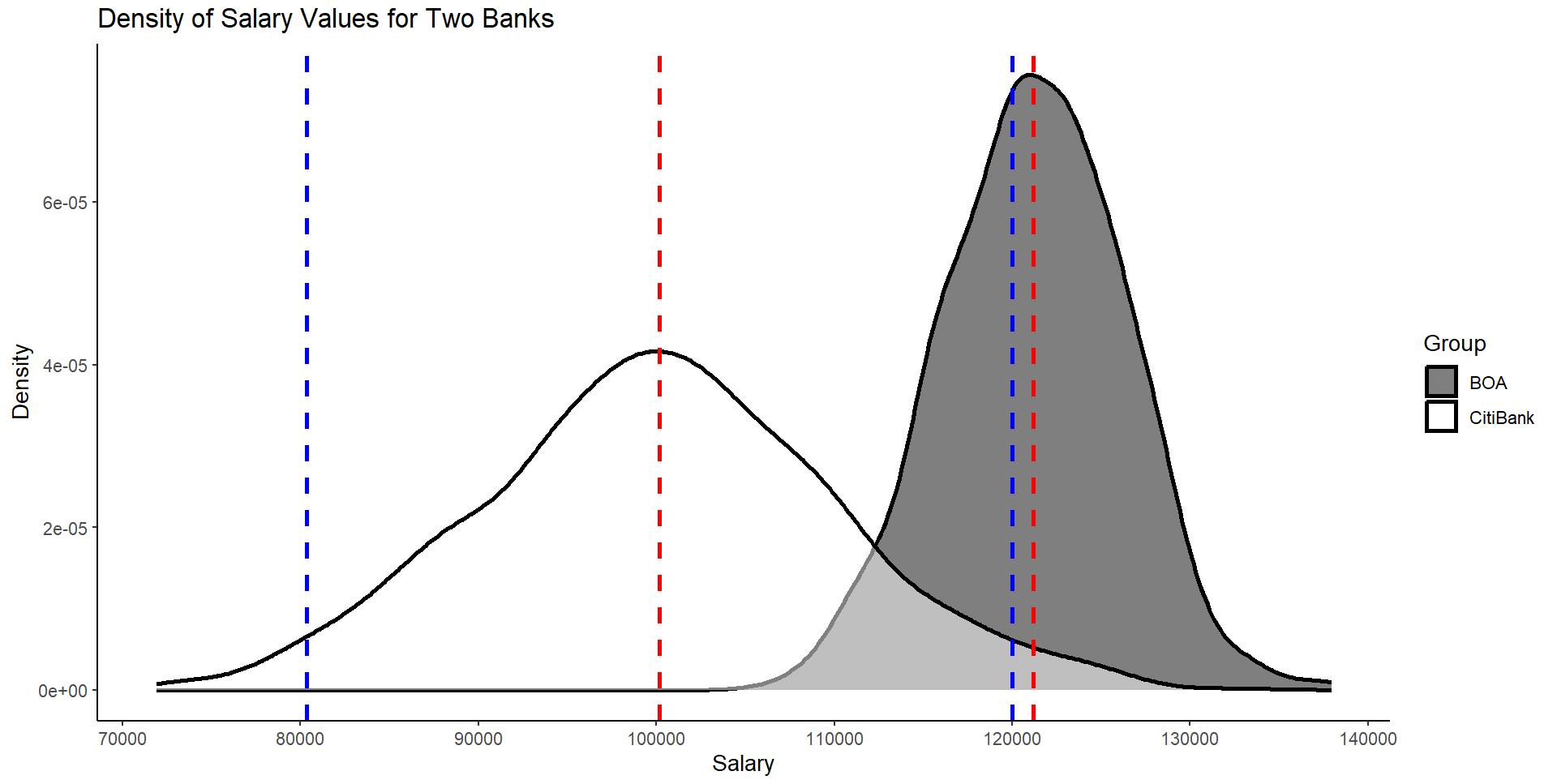
However, if we plot the critical cutoff zones used for a two-tailed test:

enter image description here

You will notice that we barely made the cutoff if using at two-tailed test (for simplicity, I just used two SD above the mean, but it should be a z-score above or below 1.96 to be precise). The red dashed lines are the means of each group and the blue dashed lines are the critical regions to reject the null.

You can see clearly that Bank of America pays more. If you were to make a judgement call about which bank to work for, which would you choose? A two-tailed test may have given you a misfire if the means were slightly different from each other. This should highlight the practicality of the test as well as why strong hypotheses are helpful to answering these questions.