deleted 25 characters in body
Source Link
Dave
  • 67.1k
  • 7
  • 105
  • 305

UNDER THE NULL HYPOTHESIS means when the null hypothesis is totally, 100% true, along with all other assumptions (such as normality for a t-test). Consequently, what ever p-values we simulate should happen for tests of true null hypothesis. In this case, we will use a one-sample t-test to test if the mean is zero, simulating independent draws from a $N(0,1)$ distribution. Thus, all standard assumptions of the t-test are satisfied: independence, equal variance, and normality. The simulation repeats this $10000$ times to get an entire distribution of p-values.

You can take it it to the extreme to see why we don't want a high $\alpha$-level: if you set $\alpha = 1$, your test always rejects. Is a rejection fromby a statistical hypothesis test that always rejects, no matter what, realany kind of evidence of a scientific (economic, whatever) discovery? I say it is not. That is equivalent to the function below that makes absolutely no use of the data.

UNDER THE NULL HYPOTHESIS means when the null hypothesis is totally, 100% true, along with all other assumptions (such as normality for a t-test). Consequently, what ever p-values we simulate should happen for tests of true null hypothesis. In this case, we will use a one-sample t-test to test if the mean is zero, simulating independent draws from a $N(0,1)$ distribution. Thus, all standard assumptions of the t-test are satisfied: independence, equal variance, and normality.

You can take it it to the extreme to see why we don't want a high $\alpha$-level: if you set $\alpha = 1$, your test always rejects. Is a rejection from a statistical hypothesis test that always rejects, no matter what, real evidence of a scientific (economic, whatever) discovery? I say it is not. That is equivalent to the function below that makes absolutely no use of the data.

UNDER THE NULL HYPOTHESIS means when the null hypothesis is totally, 100% true, along with all other assumptions (such as normality for a t-test). Consequently, what ever p-values we simulate should happen for tests of true null hypothesis. In this case, we will use a one-sample t-test to test if the mean is zero, simulating independent draws from a $N(0,1)$ distribution. Thus, all standard assumptions of the t-test are satisfied: independence, equal variance, and normality. The simulation repeats this $10000$ times to get an entire distribution of p-values.

You can take it it to the extreme to see why we don't want a high $\alpha$-level: if you set $\alpha = 1$, your test always rejects. Is a rejection by a statistical hypothesis test that always rejects, no matter what, any kind of evidence of a discovery? I say it is not. That is equivalent to the function below that makes absolutely no use of the data.

added 839 characters in body
Source Link
Dave
  • 67.1k
  • 7
  • 105
  • 305
library(ggplot2)
set.seed(2023)
N <- 1000
R <- 10000
p <- rep(NA, R)
for (i in 1:R){
  x <- rnorm(N) # Simulate the distribution
  p[i] <- t.test(x, mu = 0)$p.value # Calculate the t-test p-value
}
d0 <- data.frame(
  p_value = p,
  CDF = ecdf(p)(p),
  Distribution = "p-value Distribution"
)
d1 <- data.frame(
  p_value = p,
  CDF = qunif(p, 0, 1),
  Distribution = "U(0,1) Distribution"
)
d <- rbind(d0, d1)
ggplot(d, aes(x = p_value, y = CDF, col = Distribution)) +
  geom_line() +
  theme(legend.position="bottom")

In general, for a $U(0,1)$ distribution, if $0\le\alpha\le 1$, $P(p\le\alpha)=\alpha$. That's really the defining characteristic of the $U(0,1)$ distribution. In that sense, by picking the $\alpha$-level for the test, you pick your tolerance for rejecting when the null hypothesis is true.

However, note that rejecting in this case is a mistake. By the simulation, the null hypothesis is correct, and rejecting the null hypothesis is a so-called type I error. Errors are bad, and we like to minimize them. Consequently, it is typical to set $\alpha$ low, often around $0.05$ or lower, in order to keep from having a bunch of false positives.

You can take it it to the extreme to see why we don't want a high $\alpha$-level: if you set $\alpha = 1$, your test always rejects. Is a rejection from a statistical hypothesis test that always rejects, no matter what, real evidence of a scientific (economic, whatever) discovery? I say it is not. That is equivalent to the function below that makes absolutely no use of the data.

worthless.test <- function(input_data){
    print("Reject the null hypothesis!")
}
library(ggplot2)
set.seed(2023)
N <- 1000
R <- 10000
p <- rep(NA, R)
for (i in 1:R){
  x <- rnorm(N) # Simulate the distribution
  p[i] <- t.test(x, mu = 0)$p.value # Calculate the t-test p-value
}
d0 <- data.frame(
  p_value = p,
  CDF = ecdf(p)(p),
  Distribution = "p-value Distribution"
)
d1 <- data.frame(
  p_value = p,
  CDF = qunif(p, 0, 1),
  Distribution = "U(0,1) Distribution"
)
d <- rbind(d0, d1)
ggplot(d, aes(x = p_value, y = CDF, col = Distribution)) +
  geom_line() +
  theme(legend.position="bottom")

In general, for a $U(0,1)$ distribution, if $0\le\alpha\le 1$, $P(p\le\alpha)=\alpha$. That's really the defining characteristic of the $U(0,1)$ distribution. In that sense, by picking the $\alpha$-level for the test, you pick your tolerance for rejecting when the null hypothesis is true.

However, note that rejecting in this case is a mistake. By the simulation, the null hypothesis is correct, and rejecting the null hypothesis is a so-called type I error. Errors are bad, and we like to minimize them. Consequently, it is typical to set $\alpha$ low, often around $0.05$ or lower, in order to keep from having a bunch of false positives.

You can take it it to the extreme to see why we don't want a high $\alpha$-level: if you set $\alpha = 1$, your test always rejects. Is a rejection from a statistical hypothesis test that always rejects, no matter what, real evidence of a scientific (economic, whatever) discovery? I say it is not. That is equivalent to the function below that makes absolutely no use of the data.

worthless.test <- function(input_data){
    print("Reject the null hypothesis!")
}
Source Link
Dave
  • 67.1k
  • 7
  • 105
  • 305

UNDER THE NULL HYPOTHESIS, THE P-VALUE HAS A UNIFORM(0,1) DISTRIBUTION.

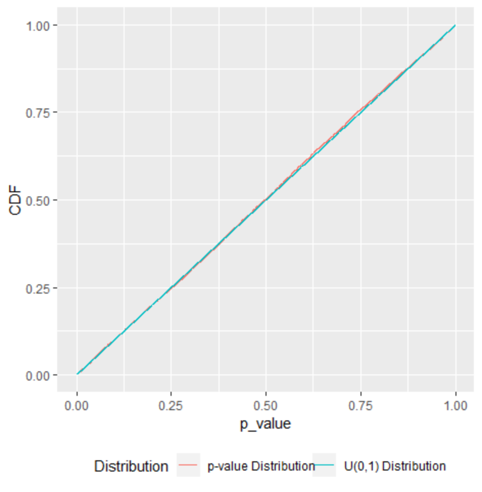
That's really all there is to it, but I believe that a simulation and a picture can help unpack that sentence.

UNDER THE NULL HYPOTHESIS means when the null hypothesis is totally, 100% true, along with all other assumptions (such as normality for a t-test). Consequently, what ever p-values we simulate should happen for tests of true null hypothesis. In this case, we will use a one-sample t-test to test if the mean is zero, simulating independent draws from a $N(0,1)$ distribution. Thus, all standard assumptions of the t-test are satisfied: independence, equal variance, and normality.

library(ggplot2)
set.seed(2023)
N <- 1000
R <- 10000
p <- rep(NA, R)
for (i in 1:R){
  x <- rnorm(N) # Simulate the distribution
  p[i] <- t.test(x, mu = 0)$p.value # Calculate the t-test p-value
}
d0 <- data.frame(
  p_value = p,
  CDF = ecdf(p)(p),
  Distribution = "p-value Distribution"
)
d1 <- data.frame(
  p_value = p,
  CDF = qunif(p, 0, 1),
  Distribution = "U(0,1) Distribution"
)
d <- rbind(d0, d1)
ggplot(d, aes(x = p_value, y = CDF, col = Distribution)) +
  geom_line() +
  theme(legend.position="bottom")

Empirical and theoretical distributions of p-values

As you can see from the lines overlapping so nicely, when the null hypothesis is true and the other test assumptions are met, the p-values generated by a t-test do generate a $U(0,1)$ distribution.

What this means is that, if you reject the null hypothesis when $p\le0.05$, you will reject in $5\%$ of these cases where the null hypothesis and other test assumptions are true, since $P(p\le0.05)=0.05$. If you reject the null hypothesis when $p=0.5$, as is suggested in the OP, you will reject in $50\%$ of these cases where the null hypothesis and other test assumptions are true, since $P(p\le0.5)=0.5$.

In general, for a $U(0,1)$ distribution, if $0\le\alpha\le 1$, $P(p\le\alpha)=\alpha$. That's really the defining characteristic of the $U(0,1)$ distribution. In that sense, by picking the $\alpha$-level for the test, you pick your tolerance for rejecting when the null hypothesis is true.