I'm coming from this questionthis question in case anybody wants to follow the trail.
Basically I have a data set $\Omega$ composed of $N$ objects where each object has a given number of measured values attached to it (two in this case):
$$\Omega = o_1[x_1, y_1], o_2[x_2, y_2], ..., o_N[x_N, y_N]$$
I need a way to determine the probability of a new object $p[x_p, y_p]$ of belonging to $\Omega$ so I was advised in that question to obtain a probability density $\hat{f}$ through a kernel density estimator, which I believe I already have.
Since my goal is to obtain the probability of this new object ($p[x_p, y_p]$) of belonging to this 2D data set $\Omega$, I was told to integrate the pdf $\hat{f}$ over "values of the support for which the density is less than the one you observed". The "observed" density is $\hat{f}$ evaluated in the new object $p$, ie: $\hat{f}(x_p, y_p)$. So I need to solve the equation:
$$\iint_{x, y:\hat{f}(x, y) < \hat{f}(x_p, y_p)} \hat{f}(x,y)\,dx\,dy$$
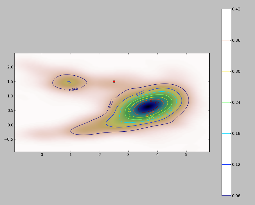
The PDF of my 2D data set (obtained through python's stats.gaussian_kde module) looks like this:

where the red dot represents the new object $p[x_p, y_p]$ plotted over the PDF of my data set.
So the question is: how can I calculate the above integral for the limits $x, y:\hat{f}(x, y) < \hat{f}(x_p, y_p)$ when the pdf looks like that?
Add
I did some tests to see how well the Monte Carlo method I mention in one of the comments worked. This is what I got:

The values appear to vary a bit more for lower density areas with both bandwidths showing more or less the same variation. The largest variation in the table occurs for the point (x,y)=(2.4,1.5) comparing Silverman's 2500 vs 1000 sample value, which gives a difference of 0.0126 or ~1.3%. In my case this would be largely acceptable.
Edit: I just noticed that in 2 dimension Scott's rule is equivalent to Silverman's according to the definition given here.
