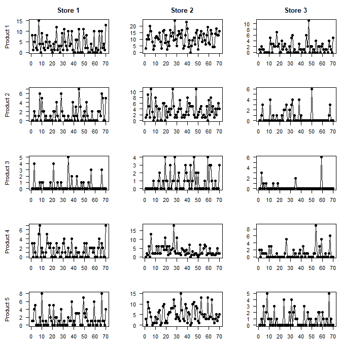
The simplest hierarchical data generating process could use a parameter $p_i$ for the $i$-th product and another parameter $s_j$ for the $j$-th store. Then you could generate data with mean $p_i+s_j$ to stand for sales of product $i$ in store $j$.

You can then expand on this in various ways.

• You could use a day of week pattern $w_{tj}$ that depends on the day of week of date $t$ (so $w_{tj}=w_{t+7,j}$) and on the store $j$, then add this to the mean: $p_i+s_j+w_{tj}$. You now have a weekly pattern that is common to all products in a store, but will differ between stores.
• Or, as for overall means, you could mix day of week patterns per store as above with another set of patterns per product, $v_{ti}$ for the $i$-th product, for a mean of $p_i+s_j+w_{tj}+v_{ti}$.
• Products are typically related hierarchically, with sales of different SKUs of milk being more closely related to each other than to sales of canned soup and diapers. You could model this by including terms that are set on various hierarchical levels.
• You could add some yearly seasonality, e.g., by including harmonics. These could again be common per store, or per product, or per product hierarchy level.
• Nothing says your terms have to be added. Multiply them together if you want.
• Sales are typically integer, so I would recommend using some count data distribution. I personally like the negative binomial.
• Especially if you use the negbin, it's natural to use a log link, by having each day's mean sales be $\exp f_{tij}$, however you calculated the log-mean $f_{tij}$ per day, product and store.

Here are some sales with $\mu_{tij}=\exp(p_i+s_j+w_{tj})$, i.e., we have a store-level day of week pattern:

R code:

n_stores <- 3
n_products <- 5
n_weeks <- 10
nb_overdispersion <- 2  # >1

set.seed(1)
store_levels <- rnorm(n_stores)
product_levels <- rnorm(n_products)
weekday_patterns <- replicate(n_stores,rnorm(7))

sales <- list()
for ( ss in 1:n_stores ) {
    sales[[ss]] <- list()
    for ( pp in 1:n_products ) {
        mu <- exp(store_levels[[ss]]+product_levels[[pp]]+rep(weekday_patterns[,ss],n_weeks))
        size <- mu/(nb_overdispersion-1)
        sales[[ss]][[pp]] <- rnbinom(7*n_weeks,mu=mu,size=size)
    }
}

opar <- par(mfcol=c(n_products,n_stores),las=1,mai=c(.3,.6,.4,.1))
    for ( ss in 1:n_stores ) {
        for ( pp in 1:n_products ) {
            plot(sales[[ss]][[pp]],type="o",pch=19,xlab="",
                ylab=ifelse(ss==1,paste("Product",pp),""),
                main=ifelse(pp==1,paste("Store",ss),""))
        }
    }
par(opar)