replaced http://stats.stackexchange.com/ with https://stats.stackexchange.com/
Source Link
added 2793 characters in body
Source Link
Flask
  • 2k
  • 1
  • 16
  • 26

EDIT with my personal version of the answer from @StéphaneLaurent

I used the model he described to sample from a normal distribution with mean=0, between subject variance =1 and within subject error/variance= 0.1,1,10,100. A subset of the confidence intervals are shown in the left panels while the distribution of their widths is shown by the corresponding right panels. This has convinced me that he is 100% correct. However, I am still confused by my example above but will follow this up with a new more focused question.
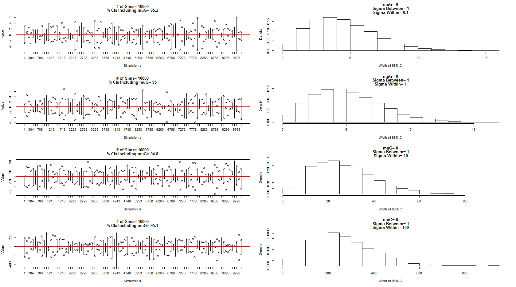
enter image description here

The code for the above simulation and charts:

dev.new()
par(mfrow=c(4,2))


num.sims<-10000
sigmaWvals<-c(.1,1,10,100)
muG<-0  #Grand Mean
sigma.between<-1  #Between Experiment sd

for(sigma.w in sigmaWvals){
  
  sigma.within<-sigma.w #Within Experiment sd
  
  out=matrix(nrow=num.sims,ncol=2)
  for(i in 1:num.sims){
    
    #Sample the three experiment means (mui, i=1:3)
    mui<-rnorm(3,muG,sigma.between)
    
    #Sample the three obersvations for each experiment (muij, i=1:3, j=1:3)
    y1j<-rnorm(3,mui[1],sigma.within)
    y2j<-rnorm(3,mui[2],sigma.within)
    y3j<-rnorm(3,mui[3],sigma.within)
    
    
    #Put results in data frame
    d<-as.data.frame(cbind(
      c(rep(1,3),rep(2,3),rep(3,3)),
      c(y1j, y2j, y3j )
    ))
    d[,1]<-as.factor(d[,1])
    
    #Calculate means for each experiment
    dmean<-aggregate(d[,2]~d[,1], data=d, FUN=mean)
    
    #Add new confidence interval data to output
    out[i,]<-t.test(dmean[,2])$conf.int[1:2]
    
  }
  
  #Calculate % of intervals that contained muG
  cover<-matrix(nrow=nrow(out),ncol=1)
  for(i in 1:nrow(out)){
    cover[i]<-out[i,1]<muG & out[i,2]>muG
  }


  sub<-floor(seq(1,nrow(out),length=100))
  plot(out[sub,1], ylim=c(min(out[sub,1]),max(out[sub,2])),
       xlab="Simulation #", ylab="Value", xaxt="n",
       main=c(paste("# of Sims=",num.sims),
              paste("% CIs Including muG=",100*round(length(which(cover==T))/nrow(cover),3)))
  )
  axis(side=1, at=1:100, labels=sub)
  points(out[sub,2])
  
  cnt<-1
  for(i in sub){
    segments(cnt, out[i,1],cnt,out[i,2])
    cnt<-cnt+1
  }
  abline(h=0, col="Red", lwd=3)
  
  hist(out[,2]-out[,1], freq=F, xlab="Width of 95% CI",
       main=c(paste("muG=", muG), 
              paste("Sigma Between=",sigma.between), 
              paste("Sigma Within=",sigma.within))
  )
  
}
tag: mixed model
Link
Stéphane Laurent
  • 19.7k
  • 5
  • 76
  • 109
Source Link
Flask
  • 2k
  • 1
  • 16
  • 26
Loading