A Bayesian approach will work as follows:
Chose a prior distribution on the number $n$ of balls in the urn. If you don't have any prior idea, you can chose the uniform distribution : $\def\P{\mathbb P}$ $$ \P_0(n = i) = {1\over 1001} \ \ (i = 0, \dots, 1000). $$
For a sample of 100 balls, denote $X$ the number of red balls. For each sample with $X=x$ update the distribution by using Bayes rule: $$ \begin{align} \P_k(n = i) &= \P_{k-1}(n = i | X = x )\\ & = \P_{k-1} (n=i) \times { \P( X= x | n = i ) \over \sum_j \P( X=x | n = j ) \P(n=j) }. \end{align}$$ Here $k$ is an index for the samples (starting from 1).
The probability $\P(X=x|n=i)$ is given by the hypergeometric distribution: $$ \P(X=x|n=i) = { {i \choose x} {1000 -i \choose 100 - x } \over {1000\choose 100} }.$$
You then have to chose a stopping criteria. You can for example stop when there is a value which has a probability > 95% (this might take a while).
Here is some R code to perform this.
# flat prior
P0 <- rep(1/1001,1001)

# updating function
update <- function(P, x)
{
  # P(X=x | n = i)
  i <- 0:1000
  Q <- dhyper(x, i, 1000-i, 100)
  # P(X=x)
  Px <- sum(Q*P)
  return( Q*P/Px )
}

X <- c(9, 10, 10, 11, 13, 8, 5, 15, 12, 9)
P <- P0;
for(x in X) P <- update(P,x)

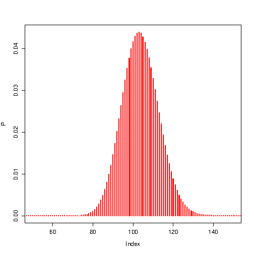
plot(P, type="h", xlim=c(50,150), col="red", lwd=2)
 ![posterior distribution][1]
[1]: https://i.sstatic.net/gWp16.png
