Is Partial Correlation useful for noisy data?

Question

Explaining The Problem

Important question in data analysis is testing observed relationships for confounding factors. Partial Correlation is a metric designed to do specifically that. The general idea is as follows. If random variables $X$ and $Y$ are correlated, but that correlation is linearly explained by another random variable $Z$, the the partial correlation between $X$ and $Y$ conditioned on $Z$, namely, $PCorr[X,Y|Z]$ should be small. More precisely, it is my intuition that partial correlation assumes the following underlying interaction model

$$X = \alpha_x Z + \nu_x$$

$$Y = \alpha_y Z + \nu_y$$

where $\alpha$ and $\beta$ are some unknown coefficients, and $\nu_x$ and $\nu_y$ are some random variables unrelated $Z$, which can be interpreted as noise or unrelated effects within $X$ and $Y$. If $\nu_x$ and $\nu_y$ were 0, then we would observe 100% correlation, and no partial correlation.

However, in realistic scenarios it frequently happens that the estimate of the confounding variable itself is a noisy function of the true confounding variable. Frequently, the actual interaction model looks something like this

$$X = \alpha_x Z + \nu_x$$

$$Y = \alpha_y Z + \nu_y$$

$$Z' = \alpha_z Z + \nu_z$$

The researcher only has access to $X, Y$ and $Z'$ but not $Z$. I decided to test if partial correlation is useful at detecting conditional independence between $X$ and $Y$ in this scenario.

Simulation

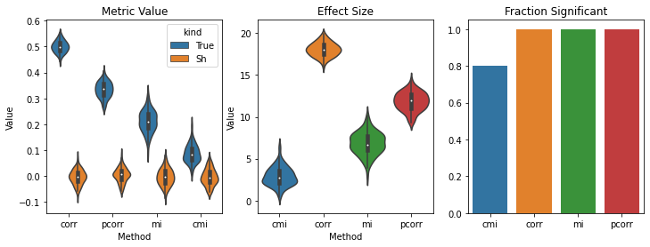
I ran a trivial simulation with $\alpha_x=\alpha_y=\alpha_z=1$, $X, Y, Z \sim \mathcal{N}(0,1)$ and $\nu_x, \nu_y, \nu_z \sim \mathcal{N}(0,1)$. I calculated correlation and partial correlation, as well as their non-linear extensions - mutual information (mi) and conditional mutual information (cmi).

I repeated the simulation 100 times, and used 1000 samples for each of the random variables $X$, $Y$ and $Z'$ for each simulation. For each simulation I computed 1 value of the metric for the simulated data, and one value for shuffled $Y$-values. The first plot shows the values of each metric for true and shuffled data - each violin is an empirical distribution over 100 points. For the second plot I estimated the effect size of each of the true datapoints using the mean and the variance of the shuffled datapoints. For the third plot, I approximated the fraction of simulations one would typically consider significant by counting the fraction of effect sizes above 2.

It is expected that correlation and mutual information would result in highly significant effects, since $X$ is indeed correlated to $Y$. However, it is unexpected (at least to me) that partial correlation and conditional mutual information are still very significant, even though their effect sizes are lower than those of correlation and mutual information respectively.

My Questions:

• Is this behaviour expected? Most literature I have seen on partial correlation does not explicitly mention that the conditional variable is not allowed to be noisy (please correct me if I'm wrong).
• Why does this happen? Can PCorr or CMI deal with this scenario at least asymptotically?
• Is the problem of discriminating between true and conditional linear dependence asymptotically solvable at all?

Jupyter notebook of the calculation is available, I will find a way to share it if there is demand

Edit 1: Theoretical Analysis

I have just performed the theoretical analysis for the noisy model, and it seems that indeed it behaves really badly even in the asymptotic case.

1. Residual is a linear fit of variable $Z'$ to variable $X$, namely $$X_{res} = X + kZ'$$ for some constant $k$, typically obtained using linear regression.

2. Partial correlation is the normalized covariance between $X_{res}$ and $Y$. We can calculate this covariance. For simplicity assume that all random variables have zero mean.

$$ \begin{eqnarray} Cov(X_{res}, Y) &=& \langle (X + kZ) Y \rangle \\ &=& \langle (\alpha_x Z + \nu_x + k(\alpha_z Z + \nu_z)) (\alpha_y Z + \nu_y) \rangle \\ &=& \langle ( (\alpha_x + k \alpha_z) Z + \nu_x + k\nu_z) (\alpha_y Z + \nu_y) \rangle \\ &=& \alpha_y (\alpha_x + k \alpha_z) Var(Z) + Cov(\nu_x, \nu_y) + kCov(\nu_z, \nu_y) \end{eqnarray} $$

Naively, we would have expected only the 2nd term in this equation, namely, the covariance between the parts of $X$ and $Y$ that are independent of $Z$. This indeed would be the case if $\nu_z$ was zero. However, we are interested to estimate what is the impact of non-zero $\nu_z$ on our estimate. There are two glaring problems. Firstly, as soon as $k$ is something different from zero, the partial correlation gets contaminated by the third term - covariance between $\nu_y$ and $\nu_z$. This is logical - by fitting $Z'$ to $X$, we to some extent remove redundant commonalities between $X$ and $Y$, but instead contaminate result with commonalities between $X$ and $Z$ that weren't there before. The second problem is the actual value of $k$. Naively, we would expect that the linear regression would be able to find the coefficient $k = -\frac{\alpha_x}{\alpha_z}$. Instead, we can estimate the asymptotic value of $k$ by minimizing the expected variance

$$L^2(k) = \langle|X_{res}|\rangle = ... = Var(\nu_x) + k Var(\nu_y) + (\alpha_x + k \alpha_z)^2 Var(S)$$

MLE estimator of $k$ for this loss function (the quantity estimated by partial correlation) can be shown to be:

$$k_{MLE} = -\frac{Cov(\nu_x, \nu_z) + \alpha_x \alpha_z Var(Z)}{Var(\nu_z) + \alpha_x^2 Var(Z)}$$

Again, if $\nu_z = 0$, the asymptotic estimate for $k_{MLE}$ converges to the expected $k = -\frac{\alpha_x}{\alpha_z}$. However, in presence of noise in $Z'$ or unique correlants between $X$ and $Z'$ the linear regression estimate for the residual is further biased.

Conclusion:

Currently this looks very bad. Guaranteeing zero noise covariate is unfeasible in many cases. Any extra components in the covariate will likely cause partial correlation to spuriously report statistically significant result for a relationship between two variables controlled for the 3rd variable, when in reality the result is redundant over all three variables and should disappear when controlled for. Please tell me that this result is well-known and I just overlooked it. The ramifications of this on already existing experimental applications of partial correlations may be huge.

Answer 1

You are correct: if the covariate is not known precisely but only as a noisy estimate, then partial correlations cannot rule out a confounding effect of the true covariate. This is an instance of the more general problem of errors-in-variables. Another common example is if you want to fit a regression model $Y=\beta X+\epsilon$, but you only have access to a noisy estimate $X'=X+\nu$. The regression or correlation coefficient resulting from such an analysis will tend to underestimate the strength of the true relationship between $X$ and $Y$, and the degree of underestimation depends on the variance of $\nu$.

This situation is accounted for by errors-in-variables models, which try to model the uncertainty in the independent variables, and thus correct the estimates of their relationships to the dependent variable(s) (and/or to each other). Some of these methods require that you know the variance of the noise in your estimates of these variables. Others try to get around that requirement. I'm not an expert on this topic but the Wikipedia article I linked should be a good starting point.

In any case, the answer is that yes, this is a known problem. Whether it is always properly appreciated by practitioners is another question of course. It is quite likely that some people are misinterpreting partial correlations when covariates are noisy. Like any statistical method, it may be misunderstood and misused. How common this is, is hard to say. I would hope that most serious data analysts will realize, through common sense, that if you don't really know the values of your covariate, then you cannot rule out that it is a confounding factor.

It is also hard to say how often this truly is a problem. Strictly speaking, it may never be possible to obtain truly error-free measurements of any variable. However, the question is whether the errors are of a meaningful magnitude. For instance, if the variance of your $\nu_z$ is non-zero, but much smaller than the variances of $X$ , $Y$ and $Z$, then technically your analysis will still be biased, but the bias will probably be negligible. Ideally, you would do some formal analysis based on an upper-bound estimate of this noise variance, to determine how serious of a problem this is. In practice, I wager this is often done in a more "seat-of-the-pants" fashion, with practitioners using their intuition to determine whether there is sufficient noise in their measurements to pose a problem to their statistical inferences.