As you said, it is difficult to find the maximum likelihood under the compound hypothesis $H:\lambda_1>\lambda_2$.
Generally, finding the maximum is often not possible in the standard way for compound hypotheses that cover only a part of the parameter space.
It can sometimes help to reparametrize - also here, as you will see later. We have the likelihood
$$
\mathcal{L}(\lambda_1, \lambda_2; x_1, x_2)=
\frac{\mathrm{e}^{-\lambda_1} \lambda_1^{x_1}}{x_1!}\cdot
\frac{\mathrm{e}^{-\lambda_2} \lambda_2^{x_2}}{x_2!}
$$
but for convenience, we maximize the log likelihood instead,
$$
\log\mathcal{L}(\lambda_1, \lambda_2; x_1, x_2)=
-(\lambda_1+\lambda_2) + x_1\log\lambda_1 + x_2\log\lambda_2 - \log(x_1!x_2!).
$$
By standard calculus, we find that this function is maximized over the unconstrainted parameter space, $(\lambda_1,\lambda_2)\in \mathbb{R}^+\times\mathbb{R}^+$, for $\hat{\lambda}_1=x_1$ and $\hat{\lambda}_2=x_2.$
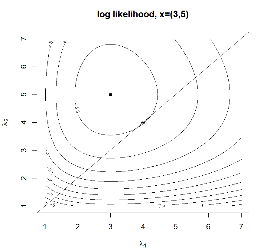
The figure below shows a contour plot of the log likelihood for $x_1=3, x_2=5$. The black dot is the maximum likelihood estimator for the unconstrainted case. Under the null hypothesis, we require $\lambda_1>\lambda_2$: this is the region under the identity line. The maximizer for this region is depicted as a circle with a cross.

How do we find that maximizer?
Notation becomes a bit less cluttered, if we write $\lambda := \lambda_1$ and $\rho := \lambda_2/\lambda_1$, that is, $\lambda_2=\rho\lambda$. Since the term $\log(x_1!x_2!)$ does not change the maximizer, we will then find the values $\rho, \lambda)$ that maximize
$$
h(\lambda, \rho) = - \lambda(1+\rho) + x_1\log \lambda + x_2\log(\lambda\rho)
$$
We find the root of
$$
\frac{\partial h(\lambda,\rho)}{\partial\lambda}=-(1+\rho)+\frac{x_1+x_2}{\lambda}=0
$$
as
$$\hat\lambda = \frac{x_1+x_2}{1+\rho},$$
and double checking the second partial derivative of $h$, we convince ourselves that this is actually a maximizer. Plugging it in to $h$, we get
$$
h(\hat\lambda,\rho)=x_2\log\rho - (x_1+x_2)\log(1+\rho)-(x_1+x_2)+(x_1+x_2)\log(x_1+x_2),
$$
and from there
$$
\frac{\partial h(\hat\lambda,\rho)}{\partial \rho}=\frac{x_2}{\rho}
-\frac{x_1+x_2}{1+\rho}=\frac{x_2-\rho x_1}{\rho(1+\rho)}.
$$
The function $\rho\to h(\hat\lambda,\rho)$ takes one local maximum in
$$\hat\rho = x_2/x_1.$$
Under the constraint $\lambda_1 > \lambda_2$, only values $\rho < 1$ are admitted.
- If $x_1>x_2$, then $\hat\rho = x_2/x_1$ is the maximizer also under the constraint, and we get
$$\hat\lambda_1 = x_1\quad \text{and}\quad \hat\lambda_2 = x_2.$$
- If $x_1\leq x_2$, then the local maximizer $x_2/x_1 \geq 1$. As $h$ is increasing in $\rho$ for $\rho\leq 1 \leq x_2/x_1$, choose $\hat\rho$ as large as allowed, so here: $\hat\rho = 1$, which gives
$$ \hat\lambda_1 = \hat\lambda_2 = (x_1 + x_2)/2. $$
Remarks on the Likelihood ratio itself
The alternative to $H_0:\lambda_1>\lambda_2$ is, strictly spoken $H_A: \lambda_1 \leq \lambda_2$. When you choose the complete parameter space instead, you would get likelihood ratio equal to 1 whenever $x_1\geq x_2$.
For one sided null hypotheses $\lambda_1 > \lambda_2$ or $\lambda_2 > \lambda_1$ and opposite alternative, nominator and denominator swap their place in the two cases $x_1>x_2$ and $x_1 < x_2$. When $x_1=x_2$, the likelihood ratio is 1.
You can easily adapt the calculations to nulhypoteses of the form $\lambda_1> 10 \lambda_2$ or $\lambda_1 < 1.5 \lambda_2$.
Code for the figure (R)
# countour plot of Poisson log likelihood

loglik <- function(lambda1, lambda2, x = c(3,5))
  dpois(x[1], lambda1, log = TRUE)+ dpois(x[2], lambda2, log = TRUE)

la1 <- seq(1, 7, 0.01)
la2 <- la1

ll <- outer(la1, la2, loglik)

# draw contour map of log likelihood function
contour(la1, la2, ll, method = "edge",
        xlab = expression(lambda[1]),
        ylab = expression(lambda[2]),
        main="log likelihood, x=(3,5)")

# unconditional maximum likelihood estimate at x
points (3, 5, pch = 16)

# identity line separating Omega_0 and Omega_1
abline(0, 1)
# conditional maximum likelihood: local maximum at (4,4)
points(4, 4, pch = 10)


self-studytag. $\endgroup$