PIT on a sample with m bins, and KS test used to estimate a good value for m

Question

I know about PIT, but this works only when you know the distribution, or at least have a strong hint. What I am trying to achieve is to transform a given sample into an equivalent sample with continuous standard uniform distribution.

I have a sample of size $n$. I choose arbitrary a value $m$, and estimate $m+1$ quantiles (for example, if $m=4$, I compute quantiles for $\{0, .25, .5, .75, 1\}$). The procedure is described in Wikipedia.

Using quantiles I transform each $x_i$. If $x_i$ happens to be exactly a computed quantile, than I know precisely its equivalent value, otherwise I interpolate the equivalent value linearly.

I've done a small simulation. I build a random sample from standard normal with $10^6$ values. I applied the described transformation and make KS test for some values of $m$. The results looks like:

  m         D   p-value
100  0.006090   0.000000000000 ***
200  0.003151   0.000000004733 ***
300  0.001991   0.000720875707 ***
400  0.001484   0.024403417075 *
500  0.001057   0.213437843144

It looks like I can do a PIT on sample with only 500 interpolation points.

The question is: can I use Kolmogorov-Smirnov one sample goodness-of-fit to find a proper value for $m$ (the number computed quantiles)?

Answer 1

The question is about applying a transformation to a given sample to obtain the corresponding sample with continuous standard uniform distribution.

I'll start by describing a natural and convenient approach to perform this type of transformation, and provide an example of the method with data considered by the OP using R. Then, I'll briefly discuss the approach considered by the OP using a quantile transformation based on subsamples.

Non-parametric transformation

A natural way to apply the probability integral transform without specifying a parametric distribution is to use the empirical distribution function (ECDF).

To avoid boundary problems, it is more convenient to use the modified empirical distribution function $$ F_n(x) = \frac{1}{n+1}\sum_{i = 1}^n I_{\{x_i\leq x\}} , $$ where $I(\cdot)$ denotes the indicator function. Applying the probability integral transform to the dataset $X_1, \ldots, X_n$ using $F_n$ corresponds to compute the normalized ranks $$ U_i = \frac{R_i}{n+1} , $$ where $R_i$ denotes the rank of $X_i$ in increasing order (i.e., $R_k = 1$ if $X_k$ is the smallest observation).

Example

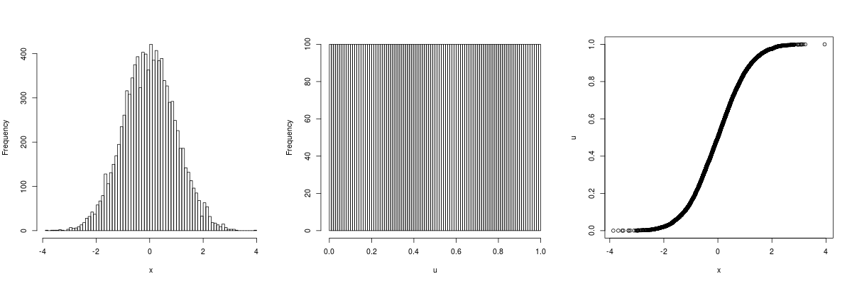
The following figure shows a histogram of the simulated dataset of $10^4$ values from the standard normal distribution (left), a histogram of the transformed data (middle), and the transformed values $U_i$ versus the original values $X_i$ (right). By construction the distribution of the transformed variables is uniform between 0 and 1.

The R code used to run this simulation is shown below.

## Parameters
n <- 10000
## Data set generation
set.seed(345)
x <- rnorm(n)
## Transformation
u <- rank(x) / (n + 1)
## Result visualization
par(mfrow = c(1, 3))
hist(x, breaks = 101, main = "")
hist(u, breaks = 101, main = "")
plot(x, u)
par(mfrow = c(1, 1))

Comments

Alternative estimates of the underlying cumulative distribution function could also be used (see here for a discussion).

The quantile-based transformation with interpolation considered by the OP is an option which corresponds to a "smoothed" version of the ECDF. However, this approach discards information contained in the dataset since it uses $m<n$ observations, resulting in a less efficient estimator of the underlying distribution. Increasing $m$ improves the quality of the estimator, so chosing $m=n$ seems most appropriate.