Analyse ACF and PACF plots

Question

I want to see if I am on the right track analysing my ACF and PACF plots:

enter image description here

Background: (Reff: Philip Hans Franses, 1998)

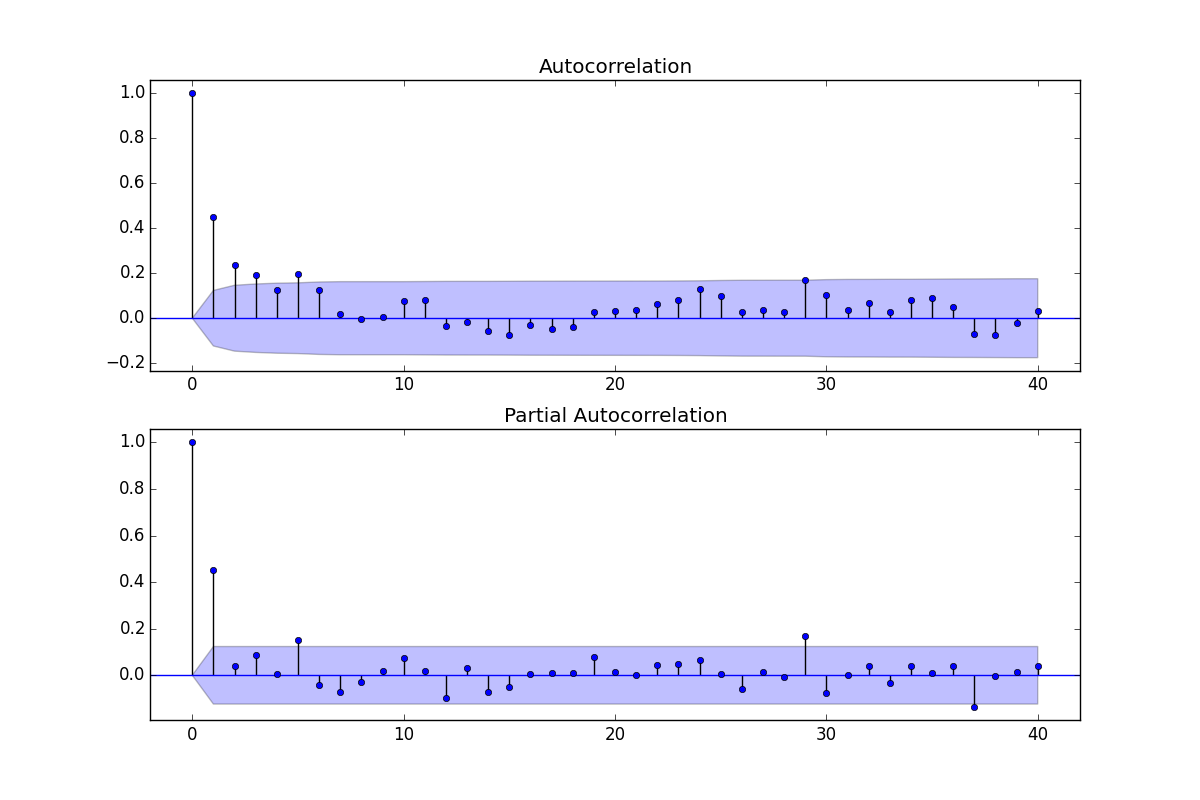
As both ACF and PACF show significant values, I assume that an ARMA-model will serve my needs
The ACF can be used to estimate the MA-part, i.e q-value, the PACF can be used to estimate the AR-part, i.e. p-value
To estimate a model-order I look at a.) whether the ACF values die out sufficiently, b.) whether the ACF signals overdifferencing and c.) whether the ACF and PACF show any significant and easily interpretable peaks at certain lags
ACF and PACF might suggest not only one model but many from which I need to choose after considering other diagnostic tools

Having that in mind, I would go ahead and say that the most obvious model seems to be ARMA (4,2) as ACF values die out at lag 4 and PACF shows spikes at 1 and 2.

Another way to analyze would be an ARMA(2,1) as I see two significant spikes in my PACF and one significant spike in my ACF (after which the values die out starting from a much lower point (0.4)).

Looking at my in-sample-forecast results (using a simple Mean Absolute Percentage Error) ARMA (2,1) delivers much better results then ARMA(4,2). So I use ARMA(2,1)!

Can you confirm my method and findings of analyzing ACF and PACF plots?

Help appreciated!

EDIT:

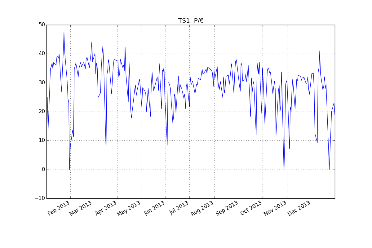
Descriptive Statistics:

count  252.000000
mean    29.576151
std      7.817171
min     -0.920000
25%     26.877500
50%     30.910000
75%     34.915000
max     47.430000

Skewness of endog_var: [-1.35798399]

Kurtsosis of endog_var: [ 5.4917757]

Augmented Dickey-Fuller Test for endog_var: (-3.76140904255411, 0.0033277703768345287, {'5%': -2.8696473721448728, '1%': -3.4487489051519011, '10%': -2.5710891239349585}

Time-Series:

enter image description here

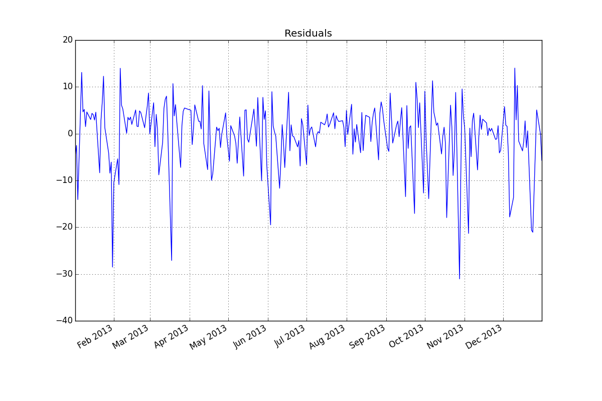
Residuals (ARMA (2,1):

enter image description here

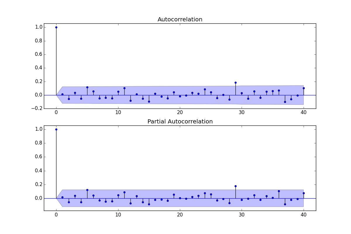
ACF/PACF of Residuals:

enter image description here

EDIT II:

Data:

Data look a bit left-skew, perhaps nonstationary. It looks to me like there's some potential issues with the residuals, perhaps even conditional heteroskedasticity. — Glen_b, Commented Jan 22, 2015 at 16:13
In my opinion the skewness suggests anomalous values (pulses) which can only be confirmed by analysis of the original data. — IrishStat, Commented Jan 22, 2015 at 21:05

kjetil b halvorsen · Accepted Answer · 2022-04-07 19:16:16Z

8

Looking at your ACF and PACF is useful in the full context of your analysis as well. Your Ljung-Box Q-statistic; p-value; confidence interval, ACF and PACF should be viewed together. For instance the Q test here:

acf, ci, Q, pvalue = tsa.acf(res1.resid, 
  nlags=4, confint=95,  qstat=True, 
  unbiased=True)

Here - our Q test for autocorrelation is an overall gut check of our graphical interpretation.

Draft notes on Time Series analysis in Statsmodels: http://conference.scipy.org/proceedings/scipy2011/pdfs/statsmodels.pdf

edited Apr 7, 2022 at 19:16

kjetil b halvorsen♦

82.8k32 gold badges201 silver badges663 bronze badges

answered Feb 20, 2015 at 23:40

unique_beast

3161 silver badge4 bronze badges

Add a comment |

IrishStat · Accepted Answer · 2015-01-24 16:53:25Z

The sole reliance on the ACF and PACF using tools suggested in the mid 60's is sometimes but seldomly correct except for simulated data. Model Identification tools like AIC/BIC almost never correctly identify a useful model but rather show what happens when you don't read the small print regarding the assumptions. I would suggest that you start as simply as possible BUT not too simply and estimate a tentative model ; AR(1) as suggested by Glen_b . The residuals/analysis from this tentative model can be used to compute yet another ACF and PACF suggesting potential model augmentation or model simplification. Note that interpretation ala your references REQUIRE that the current series/residuals are free of any deterministic structure i.e. Pulses, Level Shifts, Local Time Trends and Seasonal Pulses and furthermore that the series has constant error variance and that the parameters of the tentative model are invariant over time. If you wish you can post your data and I will attempt to help you form a useful model.

EDIT AFTER DATA WAS REPORTED :

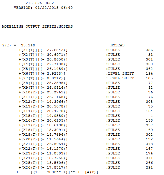365 values were delivered and analyzed, yielding the following AR(1) model with identified Pulses and 2 Level Shifts . enter image description here . note that this had been a popular guess . The residuals from this model are plotted here 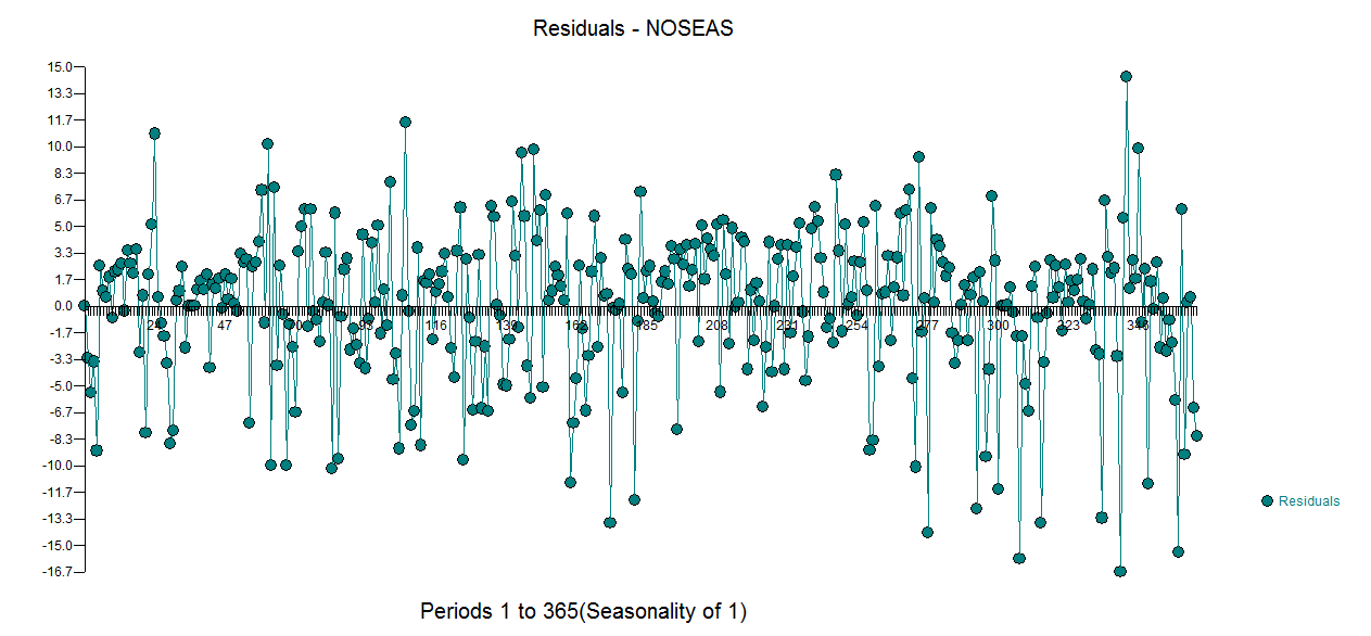. There is a suggestion of variance hetero-scedasticity but this is a symptom and one needs to find the correct cure which we will ultimately find. Proceeding the acf of the residuals shown here 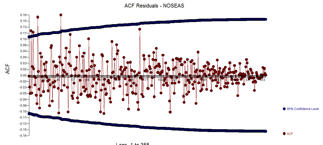enter image description here exhibits a suggestion of model inadequacy. A closer look at the table of the acf of the residuals is here 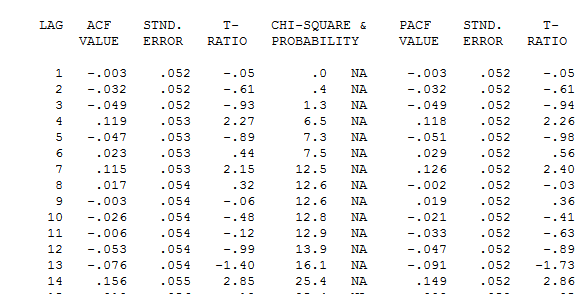suggesting structure at lags 7 and 14. Putting the the two clues together ( sample size of 365 and significant weekly i.e. lag 7 structure ) I decided to investigate whether or not this was indeed daily data. New users often omit very important information when they define their data on the mistaken premise that the computer should be smart enough to figure everything out. Note that the lag 7 and lag 14 clues were swamped in the OP'S ACF and PACF plots. The presence of deterministic structure in the residuals increase the error variance thus suppressing the acf. Once the outliers/pulses/level shifts were identified the acf revealed the presence of an autoregressive structure /daily indicators which then needed to be accounted for.

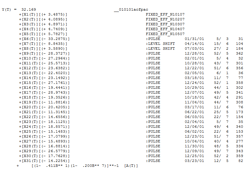I then analyzed the data allowing the software to proceed with the clue that it was daily data. With only 365 values it is not possible to properly construct models containing seasonal/holiday predictors BUT that is possible with more than 1 year of data.

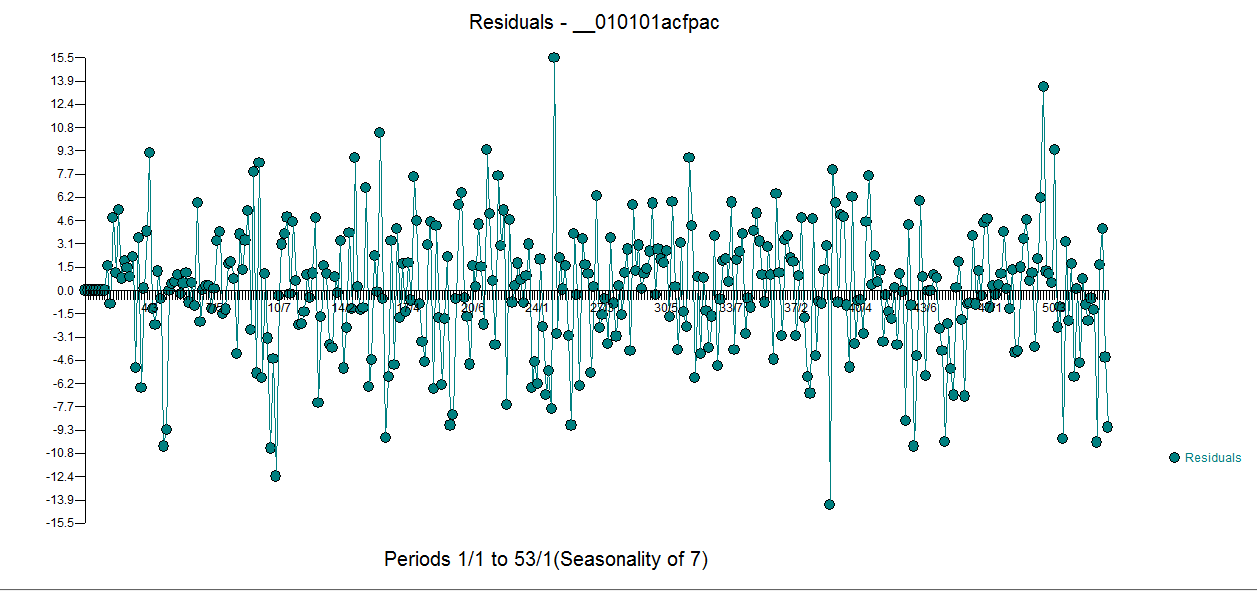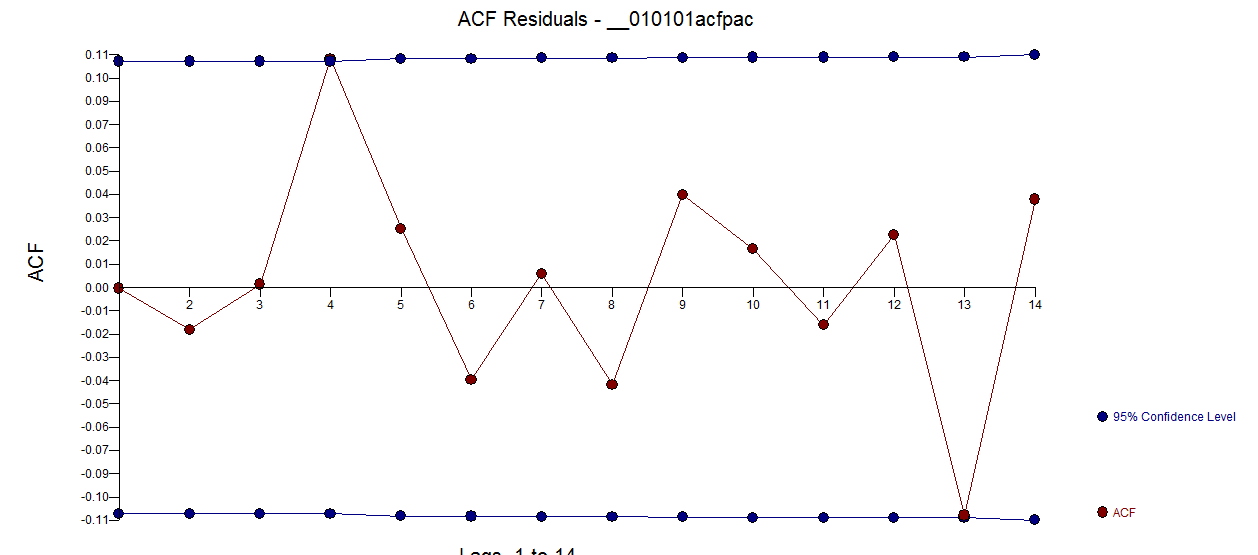The model that was found is presented here enter image description here containing 5 daily dummies , two Level Shifts , a number of pulses and an arima model of the form (1,0,0)(1,0,0) . The plot of the residuals no longer evidences the non-constancy structure as a better model is in place. . The acf of the residuals is much cleaner . The Actual /Cleansed graph highlights the unusual pulse points. 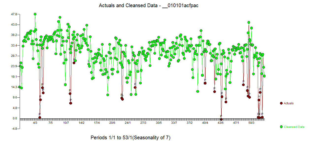enter image description here . THe lesson here is that when one analyzed the data without the critical piece of information that it was a daily time series there were a ton of pulses reflecting an inadequate representation (or perhaps the advanced knowledge of the daily clue ) . 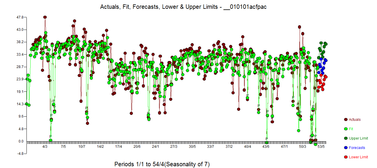The Actual/Fit and Forecast is presented here enter image description here .

It would be interesting to see what others would do with the same data set. Note that all analyses were conducted in a hands-free mode using software that is commercially available.

early morning mis read ... Don't normally see the lag(0) in my graphs — IrishStat, Commented Jan 22, 2015 at 13:45
Thanks for your answer. As someone without experience in the field of time-series forecasting it is hard to fully understand the procedure of choosing the right model as there is no officially right way to go. Unfortunately i am not allowed to post my raw data. I hope that the additional information is useful (see 'EDIT:') — Peter Knutsen, Commented Jan 22, 2015 at 14:57
You can scale/mask your data before you present it. Looking at the plot it appears there might be some unusual values which if untreated downwards biases the acf and the pacf incorrectly suggesting sufficiency. There is a visual suggestion of a downwards trend followed by no trend but that is just a guess at this moment. — IrishStat, Commented Jan 22, 2015 at 17:52

Glen_b · Accepted Answer · 2015-01-22 13:45:39Z

13

It looks to me like you're counting the spikes at lag 0.

Your PACF shows one reasonably large spike at lag 1, suggesting AR(1). This will of course induce a geometric-like decrease in the ACF (which, broadly speaking, you see). You seem to be trying to fit the same dependence twice - both as AR and MA.

I'd have just tried AR(1) on that to start with and seen if there was anything left worth worrying over.

edited Jan 22, 2015 at 13:45

answered Jan 22, 2015 at 13:34

Glen_b

290k37 gold badges652 silver badges1.1k bronze badges

$\begingroup$ Peter; my answer had a typo in it (I had AR(1) correct in the last para, but typed MA(1) in the second paragraph), which is fixed now. $\endgroup$
– Glen_b
Commented Jan 22, 2015 at 13:48
$\begingroup$ Thanks for your answer. Counting from lag 0 is of course a cardinal mistake! I tried AR(1) and the result was not as good as ARMA(2,1)! $\endgroup$
– Peter Knutsen
Commented Jan 22, 2015 at 14:26
$\begingroup$ It may well be the case that it's not as good - nevertheless, the AR(1) would be the place to start. What did the PACF of residuals look like, for example? What does the original series look like? There's much that might be going on that can't be gleaned easily from an ACF and PACF of the data. $\endgroup$
– Glen_b
Commented Jan 22, 2015 at 14:39
$\begingroup$ Thanks. I posted some additional information which might lead to new insights. $\endgroup$
– Peter Knutsen
Commented Jan 22, 2015 at 15:02

Add a comment |

Stack Exchange Network

Analyse ACF and PACF plots

3 Answers 3

Your Answer

Not the answer you're looking for? Browse other questions tagged
time-series
model-selection
arma
statsmodels
or ask your own question.

Linked

Hot Network Questions

Analyse ACF and PACF plots

3 Answers 3

Your Answer

Sign up or log in

Post as a guest

Not the answer you're looking for? Browse other questions tagged time-seriesmodel-selectionarmastatsmodels or ask your own question.

Linked

Related

Hot Network Questions

Not the answer you're looking for? Browse other questions tagged
time-series
model-selection
arma
statsmodels
or ask your own question.