Kruskal-Wallis or Fligner test to check homogeneity of variances?

Question

I need to check the homogeneity of variances on the residuals of a linear regression. I read that Kruskal is also good without assuming a normal-distribution. But I don't know if it's good in my case. I'm doing a linear regression of two vectors of prices(stock prices). I also checked the normality with Anderson-Darling test for normality (ad.test of nortest package) and the residuals seems not normally distributed, but maybe I'm choosing a wrong test to check it.

So, my goal is to check if the variance of the residuals are homogeneous. Obviously I subdivide the residuals list in two groups:

res[1:300]
res[301:600]

What can I do?

Answer 1

If I understand correctly, you have one predictor (explanatory variable $x$) and one criterion (predicted variable $y$) in a simple linear regression. The significance tests rests on the model assumption that for each observation $i$ $$ y_{i} = \beta_{0} + \beta_{1} x_{i} + \epsilon_{i} $$ where $\beta_{0}, \beta_{1}$ are the parameters we want to estimate and test hypotheses about, and the errors $\epsilon_{i} \sim N(0, \sigma^{2})$ are normally-distributed random variables with mean 0 and constant variance $\sigma^{2}$. All $\epsilon_{i}$ are assumed to be independent of each other, and of the $x_{i}$. The $x_{i}$ themselves are assumed to be error free.

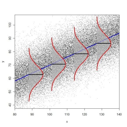
You used the term "homogeneity of variances" which is typically used when you have distinct groups (as in ANOVA), i.e., when the $x_{i}$ only take on a few distinct values. In the context of regression, where $x$ is continuous, the assumption that the error variance is $\sigma^{2}$ everywhere is called homoscedasticity. This means that all conditional error distributions have the same variance. This assumption cannot be tested with a test for distinct groups (Fligner-Killeen, Levene).

The following diagram tries to illustrate the idea of identical conditional error distributions (R-code here).

Tests for heteroscedasticity are the Breusch-Pagan-Godfrey-Test (bptest() from package lmtest or ncvTest() from package car) or the White-Test (white.test() from package tseries). You can also consider just using heteroscedasticity-consistent standard errors (modified White estimator, see function hccm() from package car or vcovHC() from package sandwich). These standard errors can then be used in combination with function coeftest() from package lmtest(), as described on page 184-186 in Fox & Weisberg (2011), An R Companion to Applied Regression.

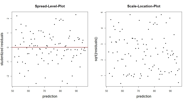
You could also just plot the empirical residuals (or some transform thereof) against the fitted values. Typical transforms are the studentized residuals (spread-level-plot) or the square-root of the absolute residuals (scale-location-plot). These plots should not reveal an obvious trend of residual distribution that depends on the prediction.

N <- 100                                  # number of observations
X <- seq(from=75, to=140, length.out=N)   # predictor
Y <- 0.6*X + 10 + rnorm(N, 0, 10)         # DV
fit   <- lm(Y ~ X)                        # regression
E     <- residuals(fit)                   # raw residuals
Estud <- rstudent(fit)                    # studentized residuals

plot(fitted(fit), Estud, pch=20, ylab="studentized residuals",
     xlab="prediction", main="Spread-Level-Plot")
abline(h=0, col="red", lwd=2)
plot(fitted(fit), sqrt(abs(E)), pch=20, ylab="sqrt(|residuals|)",
     xlab="prediction", main="Scale-Location-Plot")

Answer 2

The straightforward answer seems to be Levene's Test. Also described at Wikipedia. Levene's is applicable in your case because it is less sensitive to departures from normality than an alternative, the Bartlett Test. Levene's is parametric but suitable even with some degree of non-normality. If the distribution radically departed from normality, as with extreme outliers, you'd want to use a non-parametric alternative.

I don't see any Kruskal test as being applicable here. But you'll also want to check other threads such as this one.