0
$\begingroup$

Given $X, Y$ independent and non-normal, I'm recording histograms of $X$ and of $Z = X + Y$, sampled when $Y$ is not present and when it is, respectfully. I'm trying to figure out $Var(Y)$ and its sampling error.

I thought I could just calculate $Var(Y) = Var(Z) - Var(X)$ and use the sum of the sampling variances to produce the variance related to the final error, but the process breaks down when $Y$ is small or might not exist, occasionally resulting in a negative difference that has no meaning to me as a variance. That is, $Var(Z) - Var(X) < 0$ possibly due to sampling error.

When this difference is negative, it seems either the proposition that $Z = X + Y$ is false, or simply that the real value is close to zero and not enough samples have been taken to get the measured result close enough to zero yet.

Is there a way to determine the likelihood that the proposition is false or true when the measured value is very negative?

$\endgroup$
2
  • $\begingroup$ Deleting comments, which didn't seem to be helpful. May look at this again later. // Are you sure the $X$ you are subtracting is the same as the $X$ that is a component of $Z?$ Or do you actually have two separately-generated (therefore possible different) versions of $X$ Why can't you observe $Y$ directly? $\endgroup$
    – BruceET
    Commented Jan 13, 2019 at 20:47
  • $\begingroup$ @BruceET $X$ is almost always actually a component of $Z$, but occasionally a mistake is made and it is not, which I'd like to detect. I'm trying to remove background noise $X$ from recorded data $Y$. So I can measure the noise alone, but I can't get rid of it. // That is, X and Z are indeed separately recorded, and hence possibly different. $\endgroup$
    – fuzzyTew
    Commented Jan 13, 2019 at 20:50

3 Answers 3

1
$\begingroup$

Sample variances operate differently to the underlying variance parameters. If you would like to express the sample variance of $Y$ in terms of the sample moments of $X$ and $Z$ then you will need to formulate an appropriate decomposition formula. Assuming you are dealing with $n$ paired values (it only makes sense to add them if they are paired) you have $\bar{Y} = \bar{Z} - \bar{X}$, which then gives:

$$\begin{equation} \begin{aligned} S_Y^2 &= \frac{1}{n - 1} \sum_{i=1}^n (Y_i - \bar{Y})^2 \\[6pt] &= \frac{1}{n - 1} \sum_{i=1}^n (Z_i - X_i - \bar{Z} + \bar{X})^2 \\[6pt] &= \frac{1}{n - 1} \sum_{i=1}^n ((Z_i - \bar{Z}) - (X_i - \bar{X}))^2 \\[6pt] &= \frac{1}{n - 1} \sum_{i=1}^n \big[ (Z_i - \bar{Z})^2 - 2(Z_i - \bar{Z})(X_i - \bar{X}) + (X_i - \bar{X})^2 \big] \\[6pt] &= S_Z^2 -2 \cdot S_{X,Z} + S_X^2, \\[6pt] \end{aligned} \end{equation}$$

where we have used the sample covariance:

$$S_{X,Z} = \frac{1}{n - 1} \sum_{i=1}^n (Z_i - \bar{Z})(X_i - \bar{X}).$$

Since $Z_i = X_i + Y_i$ it is worth noting that $S_{X,Z} = S_{X,Y} + S_X^2$. Since $X$ and $Y$ are independent, as $n \rightarrow \infty$ we have $S_{X,Z} \rightarrow S_X^2$ so that $S_Y^2 \rightarrow S_Z^2 - S_X^2$.

$\endgroup$
3
  • $\begingroup$ Ben, thanks so much. Unfortunately I sample $Z$ separately from $X$, so there is not actually a pairing between the values. It would be arbitrary. It is not that I am adding them -- it is that they are produced by addition. Your example reduces to $S_Z^2 = S_Y^2 - S_X^2$ as $n \rightarrow \infty$ rather than $S_Z^2 = S_X^2 + S_Y^2$. Do you have an explanation for that? $\endgroup$
    – fuzzyTew
    Commented Jan 14, 2019 at 3:12
  • $\begingroup$ @fuzzyTew: If there is no pairing between the variables then how do you know which $X$ and $Y$ to add together to get $Z$? In any case, I have updated this answer to show the asymptotic results more clearly, which should now show why $S_Z^2 \rightarrow S_X^2 + S_Y^2$. $\endgroup$
    – Ben
    Commented Jan 14, 2019 at 4:12
  • $\begingroup$ Thanks for the changes, it makes sense now after reviewing properties of covariance. I'm learning a lot from your answer, but the X and Y are summed to Z by the underlying physical process (mixture of signal with background noise; I can only measure background noise $X$ when signal $Y$ is not present). They're not separated out per-sample. I guess I'll need a way of estimating this covariance based on properties of $X$ and $Z$. $\endgroup$
    – fuzzyTew
    Commented Jan 14, 2019 at 12:45
0
$\begingroup$

I'm tentatively considering this answer:

The likelihood I want is the likelihood that the $X$ I recorded has something in it that is not present in the $Z$ I recorded.

So if $Var(X) > Var(Z)$ I consider where in the sampling variance chi-squared distribution of Z I find $Var(X)$, and if this is beyond a threshold, I report the data as faulty.

I found a description of the sampling variance for non-normal distributions at https://stats.stackexchange.com/q/347476 . I used Wikipedia to find formulas for the variance and CDF of the chi-squared distribution: https://en.wikipedia.org/wiki/Chi-squared_distribution . I use the CDF to calculate my likelihood stat.

I would love to know whether this is correct, though!

$\endgroup$
5
  • 1
    $\begingroup$ I do not question the correctness of @Ben's Answer, to which you linked. The issue is whether it is directly applicable to your problem. The problem is somewhat simpler if $Z$ and $X$ are both normal, but even then not trivial. // In a one-way random effects ANOVA it is difficult to separate the batch component of variance from the component due to individuals from the batch. It is possible to get CIs for the intra class correlation and for the batch variance, based on F and chi-squared distributions. Gibbs sampling has been used to simulate the dist'n of the batch variance. $\endgroup$
    – BruceET
    Commented Jan 13, 2019 at 22:34
  • $\begingroup$ @BruceET Could you provide links to help someone with only introductory experience? I have billions of samples here so I should be able to pull this off. $\endgroup$
    – fuzzyTew
    Commented Jan 13, 2019 at 22:38
  • $\begingroup$ The dist'n theory is done in Gelfand and Smith (1985) JASA p398-409. Relevant Gibbs samplers are discussed in Suess (2010) Sec 9.3 (R) & 10.4 (WinBUGS). There are typos near the top of p232 corr in Suess's website errata as: $\mu^\prime = (\mu_0\theta_A + \theta_0\sum_iA_i)/(\theta_A + rg\theta_0)$ and $\theta^\prime = \theta_0\theta_A/(\theta_A + g\theta_0),$ but the R code on the text page for these formulas is OK. According to WinBUGS, it is best for priors on batch and error variances to be the same. $\endgroup$
    – BruceET
    Commented Jan 13, 2019 at 23:06
  • $\begingroup$ In a one-way random effects ANOVA, obs $Y_{ij} = \mu + A_i + e_{ij},$ where batch effect $A_i \sim \mathsf{Norm}(0, \sigma_A)$ and $e_{ij} \sim \mathsf{Norm}(0, \sigma), i = 1,\dots,g$ batches, $j = 1, \dots, n$ replications per batch. Letting $\theta_A = \sigma_A^2, \theta = \sigma^2,$ the intraclass correlation is $\rho_I = \frac{\theta_a}{\theta_A+\theta}.$ If $F$ is the var ratio for the ANOVA, then a 95% CI for $\rho_I$ is $\left(\frac{F-U}{F+(n-1)U}, \frac{F-L}{F+(n-1)L}\right),$ where $L,U$ cut 2.5% from the lower, upper tails of $\mathsf{F}(g-1,g(n-1)).$ $\endgroup$
    – BruceET
    Commented Jan 14, 2019 at 0:38
  • $\begingroup$ I'm afraid that many unexplained formulas, variables, and stats terms at once is a little too much jargon for me for now. I'll put your comments on my backburner to figure out once I get those two books off library genesis or some more stats classes. $\endgroup$
    – fuzzyTew
    Commented Jan 14, 2019 at 0:58
0
$\begingroup$

Possibly relevant simulation.

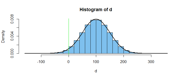
I model $S$ as the sum of ten observations from $\mathsf{Norm}(\mu=10, \sigma=5),$ corresponding to your $Z = X+Y,$ and $T$ as the sum of ten observations from $\mathsf{Norm}(9, 3),$ corresponding to your (separately observed) $X$. Then $D$ corresponds to your attempt to recover the distribution of $Y.$ However $D$ is approximately $\mathsf{Norm}(100, 50).$

This formulation models that $X$'s that are components of $S$ as independent of the $X$'s that are simulated separately as $T$'s. The $D$'s have the same mean as the $Y$'s, but not the same variance.

set.seed(113);  m = 10^6; n = 100
d = replicate(m,  sum(rnorm(n, 10, 4)) - sum(rnorm(n, 9, 3)))
mean(d);  sd(d);  mean(d < 0)
[1] 99.99261   # aprx E(D)
[1] 49.99622   # aprx SD(D)
[1] 0.022642   # aprx P(D < 0)

Notice that more than 2% of the simulated $D$'s are negative.

hist(d, prob=T, br = 25, col="skyblue2")
curve(dnorm(x, 100, 50), add=T, lwd=2)
abline(v = 0, col="green2")

enter image description here

$\endgroup$
2
  • $\begingroup$ sum(rnorm(n, 10, 4)) - sum(rnorm(n, 9, 3)) this appears to be a distribution of the difference between the two sums each of n samples taken from the two distributions. did you perhaps mean the measured variances rather than the sums, to demonstrate the error in my approach? I'm not sure I see the relevance of the difference of sums of many samples. $\endgroup$
    – fuzzyTew
    Commented Jan 14, 2019 at 0:56
  • 1
    $\begingroup$ this does show clearly that when subtracting two distributions with differing means, you can get the wrong sign in the result. $\endgroup$
    – fuzzyTew
    Commented Jan 14, 2019 at 3:23

Your Answer

By clicking “Post Your Answer”, you agree to our terms of service and acknowledge you have read our privacy policy.

Not the answer you're looking for? Browse other questions tagged or ask your own question.