3
$\begingroup$

I am trying to perform a Monte-Carlo simulation using R. Currently I am getting stuck simulating the data. In a usual regression setting I would draw a random sample of the independent data and then compute the value of my dependent variable given a set of coefficients, set by me, and an error term. Consider for example: $$ y_{i}=x_i'\beta+\epsilon_i $$ In the case of OLS the coefficient is known since I would have set it in the above equation. However, I want to compare my estimate of $\beta$ for a whole range of quantiles for example $\tau = \{0.05, 0.25, 0.5, 0.75, 0.95\}$.

So my question is, how do I simulate my data and then get my true slope parameter for all $\tau$?

$\endgroup$
3
  • 1
    $\begingroup$ I don’t follow what you’re doing, but I’ll mention that if you have $iid$ error terms, then the slope is the same at every quantile $\tau$. $\endgroup$
    – Dave
    Commented Dec 3, 2020 at 12:35
  • $\begingroup$ My problem is essentially to get a sense of how to simulate data and then know the slope parameter for the desired quantiles. So I can compare my estimate to my true parameter. $\endgroup$ Commented Dec 3, 2020 at 12:41
  • $\begingroup$ It’s going to depend on the error term. How are you simulating that? $\endgroup$
    – Dave
    Commented Dec 3, 2020 at 12:44

2 Answers 2

2
$\begingroup$

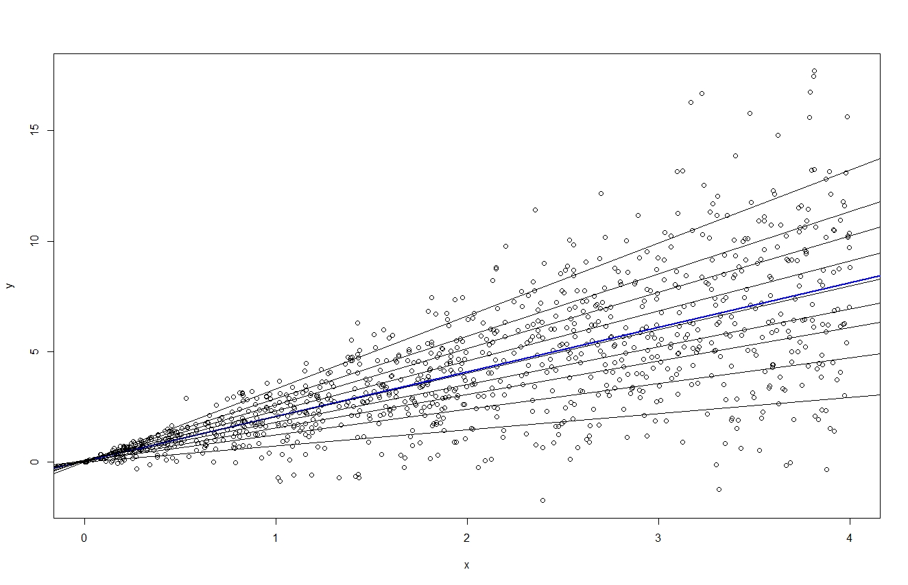
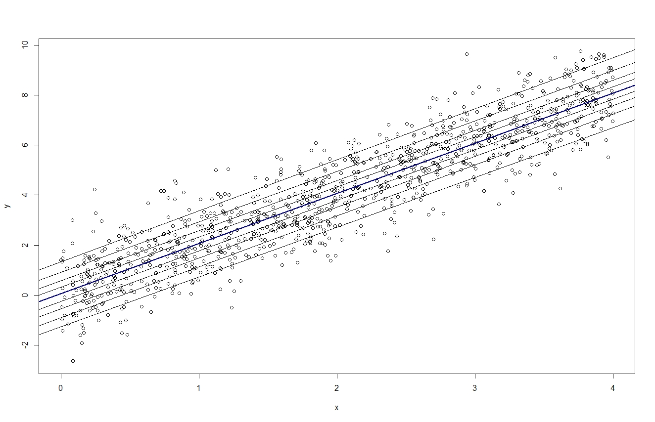
Here is a little code to get you started. It is not a simulation study, but just one run, of course. It first illustrates that there is little difference for the slopes (as Dave already said) when errors are iid, where the second example is more meaningful with heteroskedastic errors.

library(quantreg)
n <- 1000
beta <- 2

x <- runif(n, 0, 4)
u <- rnorm(n) # homoskedastic errors
y <- x*beta + u

plot(x, y)
abline(lm(y~x), lwd=2, col="blue")
rq(y~x, seq(0.1,0.9, by=0.1))
lapply(seq(0.1, 0.9, by=0.1), function(tt) abline(rq(y~x, tau=tt)))

u <- x*rnorm(n) # heteroskedastic errors
y <- x*beta + u
plot(x, y)
abline(lm(y~x), lwd=2, col="blue")
rq(y~x, seq(0.1,0.9, by=0.1))
lapply(seq(0.1, 0.9, by=0.1), function(tt) abline(rq(y~x, tau=tt)))

enter image description here

enter image description here

$\endgroup$
2
  • $\begingroup$ Thank you for your illustrative example. So to sum it up, the coefficients differ between the quantiles if heteroskedasticity is present? $\endgroup$ Commented Dec 6, 2020 at 14:17
  • $\begingroup$ Yes, that is about it, I would say! $\endgroup$ Commented Dec 7, 2020 at 4:44
1
$\begingroup$

The true slope parameter depends on the variance function. Here is some R code to illustrate.

n = 1000
beta0 = 2.1; beta1 = 0.7
set.seed(12345)
X = runif(n, 10, 20)
Y = beta0 + beta1*X + .4*X*rnorm(n)

beta1.90 = beta1 + qnorm(.90)*.4 # True slope of the .90 quantile function
beta1.90
library(quantreg)  
fit.90 = rq(Y ~ X, tau = .90)
summary(fit.90)
$\endgroup$
1
  • $\begingroup$ Thank you. That 6th command was what I was looking for! $\endgroup$ Commented Dec 6, 2020 at 14:18

Your Answer

By clicking “Post Your Answer”, you agree to our terms of service and acknowledge you have read our privacy policy.

Not the answer you're looking for? Browse other questions tagged or ask your own question.