How to calculate Hodges-Lehmann estimator of slope in rank regression?

Question

Suppose we have $n$ paired observations $(x_1,y_1),(x_2,y_2),\ldots,(x_n,y_n)$, where $y$ is the response variable and $x$ is the covariate. Consider a simple linear regression model $$y_i=\alpha+\beta x_i+\varepsilon_i\,,$$

where $\varepsilon_i$'s are i.i.d with distribution function $F$. Here $F$ has median $0$, it is absolutely continuous and unknown. We also have $x_1\le x_2\le \cdots\le x_n$, where $x_i$'s are not all equal.

Define $$T(\beta)=\sum_{i=1}^n (x_i-\overline x)R_i(\beta)\,,$$ where $R_i(\beta)$ is the rank of $y_i-\beta x_i$ for every $i$.

Hodges-Lehmann estimator of the slope $\beta$ is then $$\hat\beta_{HL}=\frac{\hat{\overline\beta}+\hat{\underline\beta}}{2}\,,$$

where $\hat{\overline\beta}=\sup\{\beta: T(\beta)>0\}$ and $\hat{\underline\beta}=\inf\{\beta : T(\beta)<0\}$.

Is there a way to calculate $\hat\beta_{HL}$ given a dataset $(x_i,y_i)$, possibly using R? The only possible way seems to be through iteration where I get an approximate solution $\hat\beta_{HL}$ (if it exists) from $T(\hat\beta_{HL})\approx 0$. This is because $T$ is actually a test statistic for testing $H_0:\beta=0$, and under $H_0$, distribution of $T$ is symmetric about $0$. But even then, I am not sure how to actually implement this.

Edit.

Consider the following data with some potential outliers:

x=c(4.37, 4.56, 4.26, 4.56, 4.3, 4.46, 3.84, 4.57, 4.26, 4.37, 
    3.49, 4.43, 4.48, 4.01, 4.29, 4.42, 4.23, 4.42, 4.23, 3.49, 
    4.29, 4.29,  4.42, 4.49, 4.38, 4.42, 4.29, 4.38, 4.22, 3.48,
    4.38, 4.56, 4.45, 3.49, 4.23, 4.62, 4.53, 4.45, 4.53, 4.43, 
    4.38, 4.45, 4.5, 4.45, 4.55, 4.45, 4.42)
    
y=c(5.23, 5.74, 4.93, 5.74, 5.19, 5.46, 4.65, 5.27, 5.57, 5.12, 
    5.73, 5.45, 5.42, 4.05, 4.26, 4.58, 3.94, 4.18, 4.18, 5.89,
    4.38, 4.22, 4.42, 4.85, 5.02, 4.66, 4.66, 4.9, 4.39, 6.05,                                          4.42, 5.10, 5.22, 6.29, 4.34, 5.62, 5.1, 5.22, 5.18, 5.57, 4.62,      5.06, 5.34, 5.34, 5.54, 4.98, 4.5) 

Based on this, the least squares estimate of $\beta$ comes out as $\hat\beta_{LS}=-0.41$, whereas the robust Theil-Sen estimate is $\hat\beta_{TS}=1.73$. I thought the Hodges-Lehmann estimator is also robust to outliers. However, following @Glen_b's approach, I seem to be getting $\hat\beta_{HL}\approx -0.48$ which is close to the non-robust LS estimate. Does this have to do with the number of outliers present in the data? Or is the Hodges-Lehmann estimator defined here supposed to be close to the usual LS estimator?

Answer 1

The basic setup is to use a robust algorithm for root finding and supply it with the function you defined. You'll need one that doesn't require a derivative (the function is not even continuous, but is monotonic, so methods like binary section should still work)

A suitable algorithm will require you to find a good starting point, and/or will require you to start by bracketing the root, which bracketing may require an initial search procedure. I sort of dodge the search for a bracket in the example below because the function I call will extend the bracket if it's insufficient (we could improve the bracketing part substantially).

Note that the root finder stops with some tolerance on the root (which you have control over in the root finding function). Because the function has jumps, the value of the function at the returned root may not seem all that "close" to 0, but it will jump to the other side of 0 with only a small shift.

Here's a quick illustration in R of putting these notions together; this can be improved and made more stable (and should if you're going to let anyone actually use this).

I haven't written this as a full function of its own - the point was just to illustrate the basic idea was implemented as I said above - but it's easy enough to wrap in a function.

(For the purpose of illustration, I'll use Brent's algorithm for the root finder and Tukey's robust line for the starting point. You could substitute other choices like - say - binary section search or ITP, and linear regression, say, for an initial guess if you wished.)

Here we just make some data to work with

    #set up some example data
    alpha<-1.4
    beta<-0.87
    x<-runif(20,3,15)
    epsilon<-rlogis(20,0,0.8)
    y<-alpha+beta*x+epsilon

We use an initial estimate to get a rough bracket on the line

    # start with a robust line (can substitute `lm` here if you want)
    #   to get a rough idea of an interval. This can be improved!
    ab<-line(x,y)$coefficients
    bi<-ab[2]

Here's the code!

    # The next two lines of code are the actual algorithm:
    #  (you may want to play with some of the other arguments 
    #  to uniroot)
    T <- function(b,y,x) {xm <- mean(x); sum((x-xm)*rank(y-b*x))}
    Tzero <- uniroot(T, interval=sort(c(0,2*bi)), y=y, x=x, 
                   extendInt="yes")
    
    b <- Tzero$root   #pull out the coefficient

Does it work?

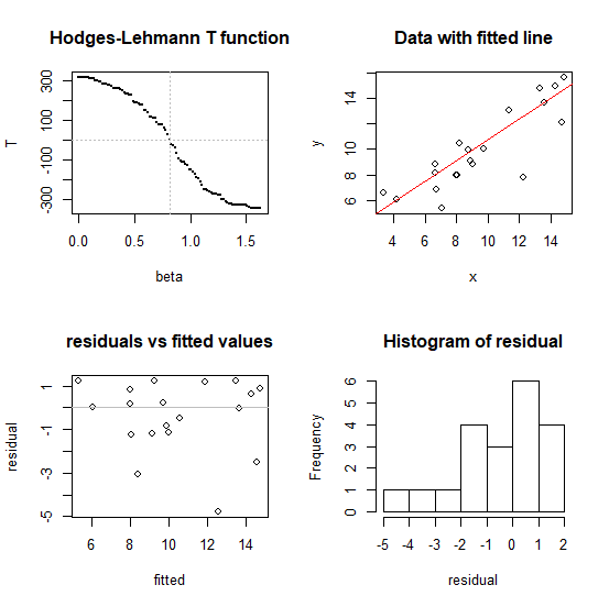
    #---- illustration of performance in four plots
    op<-par()
    par(mfrow=c(2,2))
    
    #1 don't use this normally, just to illustrate that it works
    bb<-seq(0,2*b,l=101)
    tt<-array(NA,length(bb))
    for (i in seq_along(bb)) tt[i]=T(bb[i],y,x)  
    plot(tt~bb, pch=16, cex=0.1, xlab="beta", ylab="T", 
         main="Hodges-Lehmann T function" )
    abline(h=0, v=b, col=8, lty=3)
    
    #2 
    plot(x,y,main="Data with fitted line")
    a<-median(y-b*x) # substitute whatever intercept you like
    abline(a=a,b=b,col=2)
    
    #3
    fitted<-a+b*x
    residual<-y-fitted
    plot(fitted,residual,main="residuals vs fitted values")
    abline(h=0,col=8)
    
    #4
    hist(residual)
    
    #restore plot parameters
    par(op)

Speedwise (on my fairly modest laptop) this algorithm (the two lines in the middle) finds the coefficient on a dataset with $n = 100,000$ in under a second, so it's likely to be adequate for most typical problems - but if you have very large data sets you may want to consider ways to reduce the calculation (there are ways to speed this up if it were really needed). I have tried it for $n$ up to a million (about 7 seconds to find the slope on my laptop running the code above -- but the diagnostic plots at the end took much longer, unsurprisingly). I'd hesitate to go above that sample size without more careful efforts toward speed and stability.

Note that the slope for the "Spearman line" in the answer here was also identified by root-finding (as was the quadrant-correlation slope mentioned near the end).

Answer 2

Rank regression is an informal procedure not based on a fully specified statistical model. So you can expect to have interpretation problems and especially have problems generalizing it in various ways such as adjusting for multiple covariates and incorporating repeated measures. It is better to conceptualize the problem as a semiparametric ordinal model. The proportional odds ordinal logistic regression model is one such model, and it has the Wilcoxon and Kruskal-Wallis tests as special cases. Ordinal semiparametric models allow one to obtain all sorts of predicted values included means, medians and other quantiles, exceedance probabilities, and individual cell probabilities. For details see the nonparametric statistics chapter in BBR and the long case study on ordinal models for continuous Y in RMS.

Ordinal models do not lead directly to the Hodges-Lehmann estimator but do lead directly to traditional measures such as differences in means. With some trouble you could go back to the definition of Hodges-Lehmann and derive that too, probably.