5
$\begingroup$

I would like to measure the amplitude of waves in a noisy time-series on-line. I have a time-series that models a noisy wave function, that undergoes shifts in amplitude. Say, for example, something like this:

set.seed <- 1001
x <- abs(sin(seq(from = 0, t = 100, by = 0.1)))
x <- x + (runif(1001, 0, 1) / 5)
x <- x * c(rep(1.0, 500), rep(2.0, 501))

The resulting data looks like this:

> head(x, n = 30)
 [1] 0.1581530 0.1329728 0.3911897 0.4104984 0.4774424 0.5118123 0.6499325
 [8] 0.6837706 0.8520770 0.8625692 0.8441520 0.9960601 1.1119514 1.1414032
[15] 1.1153601 1.1456799 1.0843497 1.1141201 1.1290904 0.9906415 0.9836052
[22] 0.9369836 0.9493608 0.7484588 0.7588435 0.6467422 0.5787302 0.4665009
[29] 0.4643982 0.3398427
> plot(x)
> lines(x)
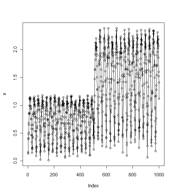
Plot of waves

As you can see, the because of the noise in the series the data does not increase monotonically between the waves' troughs and crests.

I'm looking for a way to estimate the amplitude of each wave's peak on-line in a computationally untaxing way. I can probably find a way to measure the maximum magnitude of the noise term. I'm not sure if the frequency of the waves is constant, so I'd be interested both in answers that assume a constant (known) wave frequency or a variable wave frequency. The real data is also sinusoidal.

I'm sure that this is a common problem with well-known solutions, but I am so new to this that I don't even know what terms to search for. Also, apologies if this question would be more appropriate to stackoverflow, I can ask there if that is preferred.

$\endgroup$
4
  • $\begingroup$ Are the real data also sinusoidal? Anyway, I would look into using FFT... maybe finding the max frequency with a sliding time window. $\endgroup$
    – nico
    Commented May 6, 2011 at 5:43
  • $\begingroup$ @nico Yep, updated question to say so. $\endgroup$
    – fmark
    Commented May 6, 2011 at 6:07
  • 1
    $\begingroup$ For the constant, known frequency case, it probably still breaks down further into whether you assume coherent detection or not (i.e., do you also know the phase)? At any rate, something like the empirical signal power should be close to a sufficient statistic when integrated over one period. Have you looked in, e.g., H. V. Poor, An Introduction to Signal Detection and Estimation, 2nd. ed., Springer? It almost surely does the entire development for very similar problems. $\endgroup$
    – cardinal
    Commented May 6, 2011 at 11:45
  • $\begingroup$ To follow up, in the Poor book, see the example on page 166. Of course, that particular example can be viewed in a more (statistically) "traditional" regression context. $\endgroup$
    – cardinal
    Commented May 6, 2011 at 11:55

2 Answers 2

8
$\begingroup$

More than a complete solution this is meant to be a very rough series of "hints" on how to implement one using FFT, there are probably better methods but, if it works...

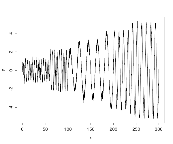
First of all let's generate the wave, with varying frequency and amplitude

  freqs <- c(0.2, 0.05, 0.1)
  x <- NULL
  y <- NULL
  for (n in 1:length(freqs))
      {
      tmpx <- seq(n*100, (n+1)*100, 0.1)
      x <- c(x, tmpx)
      y <- c(y, sin(freqs[n] * 2*pi*tmpx))
      }

  y <- y * c(rep(1:5, each=(length(x)/5)))
  y <- y + rnorm(length(x), 0, 0.2)
  plot(x, y, "l")

Which gives us this

Test wave

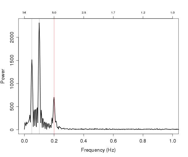
Now, if we calculate the FFT of the wave using fft and then plot it (I used the plotFFT function I posted here) we get:

Global FFT of the wave

Note that I overplotted the 3 frequencies (0.05, 0.1 and 0.2) with which I generated the data. As the data is sinusoidal the FFT does a very good job in retrieving them. Note that this works best when the y-values are 0 centered.

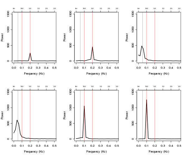
Now let's do a sliding FFT with a window of 50 we get

Windowed FFT

As expected, at the beginning we only get the 0.2 frequency (first 2 plot, so between 0 and 100), as we go on we get the 0.05 frequency (100-200) and finally the 0.1 frequency comes about (200-300).

The power of the FFT function is proportional to the amplitude of the wave. In fact, if we write down the maximum in each window we get:

1 Max frequency:  0.2  - power:  254
2 Max frequency:  0.2  - power:  452
3 Max frequency:  0.04  - power:  478
4 Max frequency:  0.04  - power:  606
5 Max frequency:  0.1  - power:  1053
6 Max frequency:  0.1  - power:  1253 

===

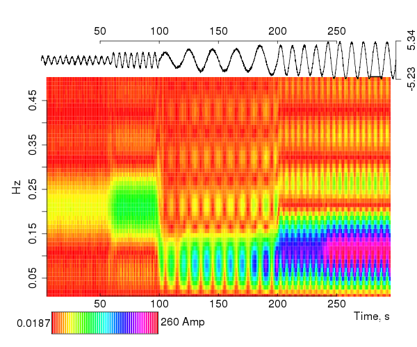
This can be also achieved using a STFT (short-time Fourier transform), which is basically the same thing I showed you before, but with overlapping windows. This is implemented, for instance, by the evolfft function of the RSEIS package.

It would give you:

stft <- evolfft(y, dt=0.1, Nfft=2048, Ns=100, Nov=90, fl=0, fh=0.5)
plotevol(stft) 

STFT

This, however, may be trickier to analyze, especially online.

hope this helps somehow

$\endgroup$
5
  • $\begingroup$ Looks to be a very good start, thank you. Not sure if its going to be too computationally taxing but I guess I'll have to try it out and see! $\endgroup$
    – fmark
    Commented May 6, 2011 at 9:43
  • $\begingroup$ @fmark: the examples I posted computed pratically istantaneously. $\endgroup$
    – nico
    Commented May 6, 2011 at 10:03
  • $\begingroup$ I will be doing this on an embedded system with limited RAM and a slow processor, and coding it myself in C, so what is instantaneous on your desktop using an optimised implementation may not be a good indication :) $\endgroup$
    – fmark
    Commented May 6, 2011 at 10:33
  • $\begingroup$ @fmark: sure, but at least you know it's not slow on a desktop!!! :D Anyway, I'm sure there's plenty of fast implementation of FFT (it's called "fast" Fourier transform for a reason). I never implemented one, though, so I cannot help in this case. $\endgroup$
    – nico
    Commented May 6, 2011 at 11:58
  • $\begingroup$ Absolutely, I'll definitely give it a try :) $\endgroup$
    – fmark
    Commented May 6, 2011 at 12:18
1
$\begingroup$

In answer to another question on this forum I referred the OP to this site where there is open source code for a function called HT_PERIOD to measure the instantaneous period of a time series. There are also functions called HT_PHASE, HT_PHASOR and HT_SINE to respectively measure the phase, the phasor components of the sine wave/cyclic component and to extract the sine wave itself (scaled between -1 and 1) of a time series. As the calculations in these functions are causal they would be appropriate for an on-line function that updates as new data comes in. The code for these functions might be of help to you.

$\endgroup$

Your Answer

By clicking “Post Your Answer”, you agree to our terms of service and acknowledge you have read our privacy policy.

Not the answer you're looking for? Browse other questions tagged or ask your own question.