Combining data from different sources

Question

I want to combine data from different sources.

Let's say I want to estimate a chemical property (e.g. a partitioning coefficient):

I have some empirical data, varying due to measurement error around the mean.

And, secondly, I have a model predicting an estimate from other information (the model has also some uncertainty).

How can I combine those two datasets? [The combined estimate will be used in another model as predictor].

Meta-analysis and bayesian methods seem to be suitable. However, haven't found many references and ideas how to implement it (I am using R, but also familiar with python and C++).

Thanks.

Update

Ok, here's a more real example:

To estimate the toxicity of a chemical (typically expressed as $LC_{50}$ = concentration where 50% of animals die) lab-experiments are conducted. Happily the results of the experiments are gathered in a database (EPA).

Here are some values for the insecticide Lindane:

### Toxicity of Lindane in ug/L
epa <- c(850 ,6300 ,6500 ,8000, 1990 ,516, 6442 ,1870, 1870, 2000 ,250 ,62000,
         2600,1000,485,1190,1790,390,1790,750000,1000,800
)
hist(log10(epa))

# or in mol / L
# molecular weight of Lindane
mw = 290.83 # [g/mol]
hist(log10(epa/ (mw * 1000000)))

However, there are also some models available to predict toxicity from chemical properties (QSAR). One of these models predicts toxicity from the octanol/water partition coefficient ($log~K_{OW}$):

$$ log~LC_{50} [mol/L] = 0.94~(\pm 0.03)~log~K_{OW}~-~1.33 (\pm~0.1)$$

The partitioning coefficient of Lindane is $log~K_{OW} = 3.8$ and the predicted toxicity is $ log~LC_{50} [mol/L] = -4.902 $.

lkow = 3.8
mod1 <- -0.94 * lkow - 1.33
mod1

Is there a nice way to combine these two different informations (lab experimens and model predictions)?

hist(log10(epa/ (mw * 1000000)))
abline(v = mod1, col = 'steelblue')

The combined $LC_{50}$ will be used later on in a model as predictor. Therefore, a single (combined) value would be a simple solution.

However, a distribution might be also handy - if this is possible in modelling (how?).

Answer 1

Your model estimate would be a useful prior.

I have applied the following approach in LeBauer et al 2013, and have adapted code from priors_demo.Rmd below.

To parameterize this prior using simulation, consider your model

$$ \textrm{logLC}_{50} = b_0 X+b_1$$

Assume $b_0 \sim N(0.94, 0.03)$ and $b_1 \sim N(1.33, 0.1)$; $\textrm{Lkow}$ is known (a fixed parameter; for example physical constants are often known very precisely relative to other parameters).

In addition, there is some model uncertainty, I'll make this $\epsilon \sim N(0,1)$, but should be an accurate representation of your information, for example the model's RMSE could be used to inform the scale of the standard deviation. I am intentionally making this an 'informative' prior.

b0 <- rnorm(1000, -0.94, 0.03)
b1 <- rnorm(1000, -1.33, 0.1)
e <- rnorm(1000, 0, 1)
lkow <- 3.8
theprior <- b0 * lkow + b1 + e

Now imagine theprior is your prior and

thedata <- log10(epa/ (mw * 1000000))

is your data:

library(ggplot2)
ggplot() + geom_density(aes(theprior)) + theme_bw() + geom_rug(aes(thedata))

The easiest way to use the prior is going to be to parameterize a distribution that JAGS will recognize.

This can be done in many ways. Since the data don't have to be normal, you might consider finding a distribution using the package fitdistrplus. For simplicity, lets just assume that your prior is N(mean(theprior), sd(theprior)), or approximately $N(-4.9, 1.04)$. If you want to inflate the variance (to give the data more strength) you could use $N(-4.9, 2)$

Then we can fit a model using JAGS

writeLines(con = "mymodel.bug",
           text = "
           model{
             for(k in 1:length(Y)) {
               Y[k] ~ dnorm(mu, tau)
             }

             # informative prior on mu
             mu ~ dnorm(-4.9, 0.25) # precision tau = 1/variance
             # weak prior 
             tau ~ dgamma(0.01, 0.01)
             sd <- 1 / sqrt(tau)
           }")

require(rjags)
j.model  <- jags.model(file = "mymodel.bug", 
                                  data = data.frame(Y = thedata), 
                                  n.adapt = 500, 
                                  n.chains = 4)
mcmc.object <- coda.samples(model = j.model, variable.names = c('mu', 'tau'),
                            n.iter = 10000)
library(ggmcmc)

## look at diagnostics
ggmcmc(ggs(mcmc.object), file = NULL)

## good convergence, but can start half-way through the simulation
mcmc.o     <- window(mcmc.object, start = 10000/2)
summary(mcmc.o)

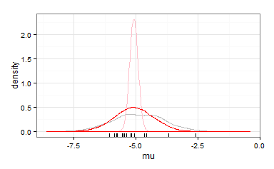
Finally, a plot:

ggplot() + theme_bw() + xlab("mu") + 
     geom_density(aes(theprior), color = "grey") + 
     geom_rug(aes(thedata)) + 
     geom_density(aes(unlist(mcmc.o[,"mu"])), color = "pink") +
     geom_density(aes(unlist(mcmc.o[,"pred"])), color = "red")

And you can consider mu=5.08 to be your estimate of the mean parameter value (pink), and sd = 0.8 its standard deviation; the posterior predictive estimate of the logLC_50 (where you are getting your samples from) is in red.

Reference

LeBauer, D.S., D. Wang, K. Richter, C. Davidson, & M.C. Dietze. (2013). Facilitating feedbacks between field measurements and ecosystem models. Ecological Monographs 83:133–154. doi:10.1890/12-0137.1