Intervention With Differencing

Question

When conducting an intervention analysis with time series data (aka Interrupted Time series) as discussed here for example one requirement I have is to estimate the total gain (or loss) due to the intervention - i.e. number of units gained or lost (the Y variable).

Not entirely understanding how to estimate the intervention function using a filter function within R, I went about it in a brute force manner, hoping this is general enough to work in any situation.

Lets say that given the data

 cds<- structure(c(2580L, 2263L, 3679L, 3461L, 3645L, 3716L, 3955L, 
    3362L, 2637L, 2524L, 2084L, 2031L, 2256L, 2401L, 3253L, 2881L, 
    2555L, 2585L, 3015L, 2608L, 3676L, 5763L, 4626L, 3848L, 4523L, 
    4186L, 4070L, 4000L, 3498L), .Dim = c(29L, 1L), .Dimnames = list(
        NULL, "CD"), .Tsp = c(2012, 2014.33333333333, 12), class = "ts")

we decide that the best fitting model is as follows, with the intervention function as

$m_t= \frac{\omega_0}{(1-\delta B)}X_t$ where $X_t$ is a pulse at October 2013.

fit4 <- arimax(log(cds), order = c(1,1,0),include.mean=FALSE, 
               xtransf = data.frame(Oct13 = 1*(seq_along(cds)==22)),
               transfer = list(c(1,0))
               ,xreg=1*(seq_along(cds)==3))
fit4

#    ARIMA(1,1,0)                    

#    Coefficients:
#              ar1    xreg  Oct13-AR1  Oct13-MA0
#          -0.0184  0.2718     0.4295     0.4392
#    s.e.   0.2124  0.1072     0.3589     0.1485

#    sigma^2 estimated as 0.02176:  log likelihood=13.85
#    AIC=-19.71   AICc=-16.98   BIC=-13.05

I have two questions:

1) Even though we have differenced the ARIMA errors , to assess the intervention function which was then technically fit using the differenced series $\bigtriangledown X_t $ is there anything we need to do in order to "change back" the estimate of $\omega_0$ or $\delta$ from using $\bigtriangledown X_t $ to $ X_t $?

2) Is this correct: In order to determine the gain of the intervention, I constructed the intervention $m_t$ from the parameters. Once I have $m_t$ then I compare the fitted values from the model fit4 (exp() to reverse the log) to exp( fitted values minus $m_t$ ) and determine that over the observed period, the intervention resulted in 3342.37 extra units.

Is this process the correct one to determine the gain generally from an intervention analysis?

    int_vect1<-1*(seq_along(cds)==22)
    wo<- 0.4392
    delta<-0.4295


    mt<-rep(0,length(int_vect1))

    for (i in 1:length(int_vect1))
    {

      if (i>1)
      {
        mt[i]<-wo*int_vect1[i]+delta*mt[i-1]
      }

    }


    mt

sum(exp(fitted(fit4)) - (exp(fitted(fit4) - mt)))

Answer 1

Assuming this is toy example:

To answer your first question:

1) Even though we have differenced the ARIMA errors , to assess the intervention function which was then technically fit using the differenced series ▽Xt is there anything we need to do in order to "change back" the estimate of ω0 or δ from using ▽Xt to Xt?

When you difference the data, you should difference the response/intervention variables. When you back difference (transform) after you model then this would automatically take care of differencing** I know this is very easy when you use SAS Proc ARIMA. I dont know how to do this R.

Second Question:

2) Is this correct: In order to determine the gain of the intervention, I constructed the intervention mt from the parameters. Once I have mt then I compare the fitted values from the model fit4 (exp() to reverse the log) to exp( fitted values minus mt ) and determine that over the observed period, the intervention resulted in 3342.37 extra units.

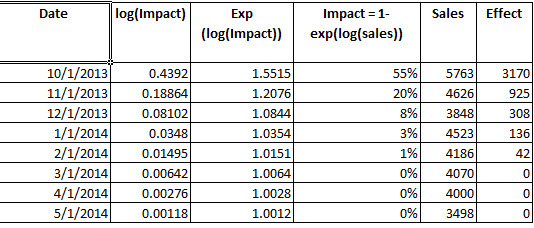
To determine, gain in intervention, you need to take exponent and then subtract -1, this would give the proportion or incremental effect. To demonstrate this in your case, see below. For the first month, the impact was 55% of original sales and rapidly decays. Cumulativelt you have 4580 units of incremental effect (Oct 13 thru Feb 2014. (I referred to Forecasting Principle and Applications by Delurgio P: 518. There is an excellent voluminous chapter on intervention analysis).

Someone please correct if this methodology is correct ?

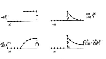
Pulse intervention + decay is clearly not sufficient in this case, I would do a pulse + permanent level shift as shown in the diagram (e) below which is from the classic paper by Box and Tiao.

Answer 2

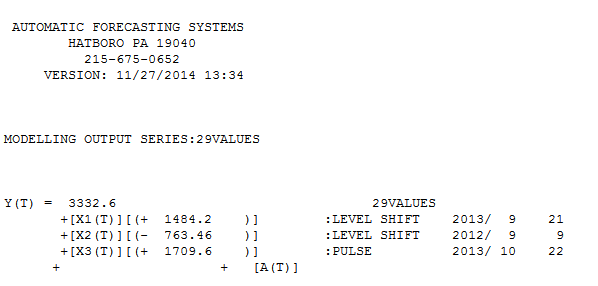
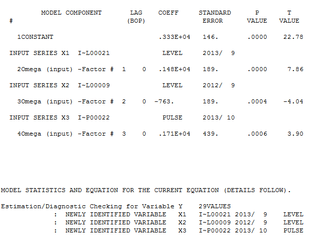
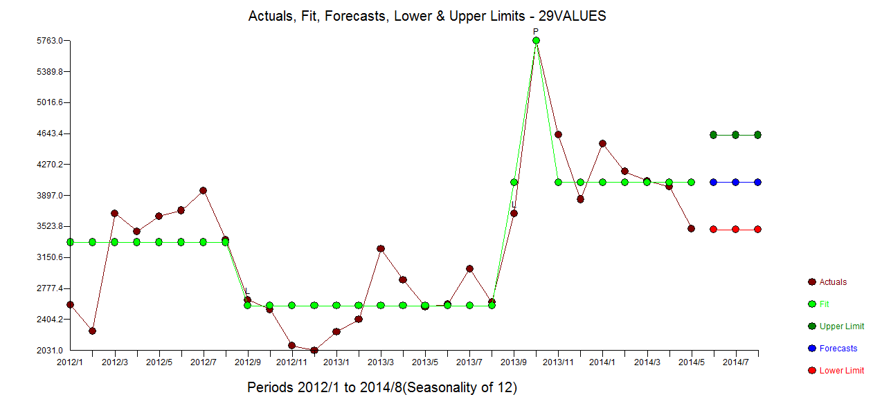
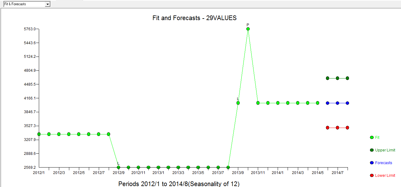
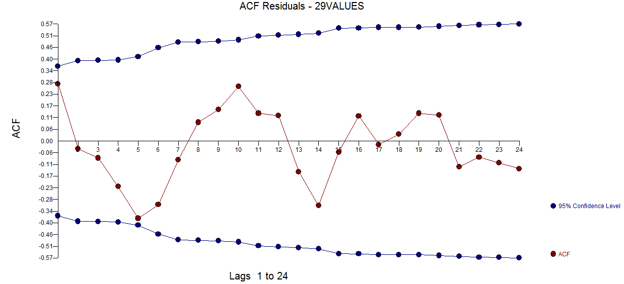
@forecaster After allowing AUTOBOX to identify 3 outliers using 29 values (not inappropriate in y experience) a useful model was found and here . The residual acf plot does not suggest an under-specified model . The Actual/Fit/Forecast plot is with Fit/Forecast here . Forecaster had (correctly) previously mentioned how a pulse variable can morph into a level/step variable when a denominator coefficient of nearly 1.0 is introduced. In finding two level shifts (the most recent one starting in 9/2013) and a pulse at 10/2013 , the model presents a clearer picture. In terms of the impact of the pulse at 10/13 it is simply the value of the coefficient. HTH