Why does the t-distribution become more normal as sample size increases?

Question

As per Wikipedia, I understand that the t-distribution is the sampling distribution of the t-value when the samples are iid observations from a normally distributed population. However, I don't intuitively understand why that causes the shape of the t-distribution to change from fat-tailed to almost perfectly normal.

I get that if you're sampling from a normal distribution then if you take a big sample it will resemble that distribution, but I don't get why it starts out with the fat-tailed shape it does.

Answer 1

I'll try to give an intuitive explanation.

The t-statistic* has a numerator and a denominator. For example, the statistic in the one sample t-test is

$$\frac{\bar{x}-\mu_0}{s/\sqrt{n}}$$

*(there are several, but this discussion should hopefully be general enough to cover the ones you are asking about)

Under the assumptions, the numerator has a normal distribution with mean 0 and some unknown standard deviation.

Under the same set of assumptions, the denominator is an estimate of the standard deviation of the distribution of the numerator (the standard error of the statistic on the numerator). It is independent of the numerator. Its square is a chi-square random variable divided by its degrees of freedom (which is also the d.f. of the t-distribution) times the square of $\sigma_\text{numerator}$.

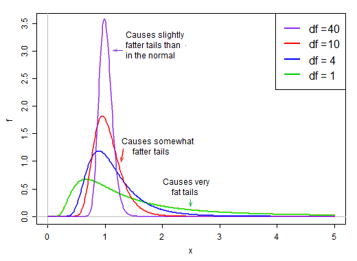
When the degrees of freedom are small, the denominator tends to be fairly right-skew. It has a high chance of being less than its mean, and a relatively good chance of being quite small. At the same time, it also has some chance of being much, much larger than its mean.

Under the assumption of normality, the numerator and denominator are independent. So if we draw randomly from the distribution of this t-statistic we have a normal random number divided by a second randomly* chosen value from a right-skew distribution that's on average around 1.

* without regard to the normal term

Because it's on the denominator, the small values in the distribution of the denominator produce very large t-values. The right-skew in the denominator make the t-statistic heavy-tailed. The right tail of the distribution, when on the denominator makes the t-distribution more sharply peaked than a normal with the same standard deviation as the t.

However, as the degrees of freedom become large, the distribution becomes much more normal-looking and much more "tight" around its mean.

As such, the effect of dividing by the denominator on the shape of the distribution of the numerator reduces as the degrees of freedom increase.

Eventually - as Slutsky's theorem might suggest to us could happen - the effect of the denominator becomes more like dividing by a constant and the distribution of the t-statistic is very close to normal.

---

Considered in terms of the reciprocal of the denominator

whuber suggested in comments that it might be more illuminating to look at the reciprocal of the denominator. That is, we could write our t-statistics as numerator (normal) times reciprocal-of-denominator (right-skew).

For example, our one-sample-t statistic above would become:

$${\sqrt{n}(\bar{x}-\mu_0)}\cdot{1/s}$$

Now consider the population standard deviation of the original $X_i$, $\sigma_x$. We can multiply and divide by it, like so:

$${\sqrt{n}(\bar{x}-\mu_0)/\sigma_x}\cdot{\sigma_x/s}$$

The first term is standard normal. The second term (the square root of a scaled inverse-chi-squared random variable) then scales that standard normal by values that are either larger or smaller than 1, "spreading it out".

Under the assumption of normality, the two terms in the product are independent. So if we draw randomly from the distribution of this t-statistic we have a normal random number (the first term in the product) times a second randomly-chosen value (without regard to the normal term) from a right-skew distribution that's 'typically' around 1.

When the d.f. are large, the value tends to be very close to 1, but when the df are small, it's quite skew and the spread is large, with the big right tail of this scaling factor making the tail quite fat:

Answer 2

@Glen_b gave you the intuition on why the t statistic looks more normal as the sample size increases. Now, I will give you a slightly more technical explanation for the case when you already got the distribution of the statistic.

It is well-known that the t-statistic is distributed as a student t dsitribution with $n-1$ degrees of freedom, where $n$ is the sample size. The corresponding density looks as follows:

$$\frac{\left(1+\frac{x^2}{n-1}\right)^{-n/2}}{\sqrt{n-1} B\left(\frac{n-1}{2},\frac{1}{2}\right)}.$$

It is possible to show that

$$\frac{1}{\sqrt{n-1} B\left(\frac{n-1}{2},\frac{1}{2}\right)}\rightarrow \frac{1}{\sqrt{2\pi}},$$

and

$$\left(1+\frac{x^2}{n-1}\right)^{-n/2}\rightarrow \exp(-x^2/2),$$

as $n\rightarrow \infty$. By taking the product of these two limits you can see that the Student-t density converges exactly to the standard normal density.

Answer 3

I just wanted to share something that helped my intuition as a beginner (though it's less rigorous than the other answers).

If $Z, Z_1, ..., Z_n$ are iid standard normal RVs then the following RV,

$$\frac{Z}{\sqrt{\frac{Z_1^2+...+Z_n^2}{n}}}$$

has a t-distribution with $n$ degrees of freedom.

As $n$ gets really big, using the law of large numbers we can see that the denominator goes to $1$. So you're just left with $Z$ which is standard normal which is why the t-distribution looks normal as $n$ gets big.

To elaborate... note that $E[Z^2] = 1$ which says the expected value of a chi squared RV is one. The fraction in the square root is just the sample mean of $n$ iid $Z_i^2$ RVs. The sample mean as $n$ gets super big will equal the expected value of just one of the $Z_i^2$'s which is one.

So as $n$ gets really big you're just left with $\frac{Z}{\sqrt{1}} = Z$