Should I use t-test on highly skewed and discrete data?

Question

I have samples from a highly skewed dataset about users' participation (e.g.: number of posts), that have different sizes (but not less than 200) and I want to compare their mean. For that, I'm using two-sample unpaired t-tests(and t-tests with the Welch’s factor, when the samples had different variances). As I have heard that, for really large samples, it doesn't matter that the sample are not normal distributed.

My metrics are discrete, they are counts of the number of each user's participation. Of course we have those users who participate much more than the others, but I'm not considering them as outliers. Here are the data description: https://docs.google.com/spreadsheets/d/1WhSKgYIuP35eRsukHVoUFUlITNwO_RRcYoOoR9EmXHg/edit?usp=sharing$^\dagger$

My problem: someone, reviewing what I've done, said that the tests I am using were not suitable for my data. They suggested to log-transform my samples before using the t-tests.

I do know that I can't log-transform these, because all of them have zero-values on the samples. My guess is, if I can't use t-test, I should use the Mann Whitney U test.

Are they wrong? Am I wrong? If they are wrong, is there a book or scientific paper which I could cite/show them? If I am wrong, which test should I use?

--

$\dagger$ link not active

Answer 1

Highly discrete and skew variables can exhibit some particular issues in their t-statistics:

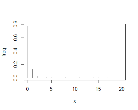
For example, consider something like this:

(it has a bit more of a tail out to the right, that's been cut off, going out to 90-something)

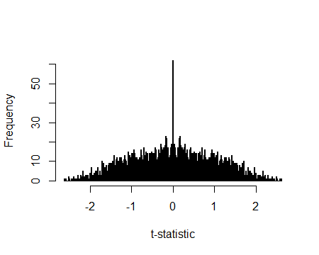
The distribution of two-sample t-statistics for samples of size 50 look something like this:

In particular, there are somewhat short tails and a noticeable spike at 0.

Issues like these suggest that simulation from distributions that look something like your sample might be necessary to judge whether the sample size is 'large enough'

Your data seems to have somewhat more of a tail than in my above example, but your sample size is much larger (I was hoping for something like a frequency table). It may be okay, but you could either simulate form some models in the neighborhood of your sample distribution (or you could resample your data) to get some idea of whether those sample sizes would be sufficient to treat the distribution of your test statistics as approximately $t$.

---

Simulation study A - t.test significance level (based on the supplied frequency tables)

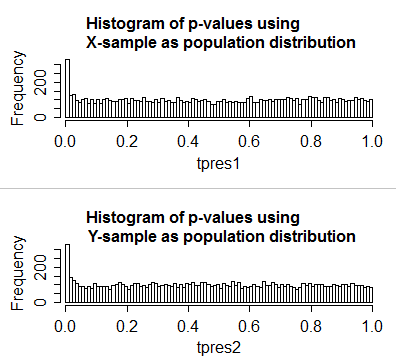
Here I resampled your frequency tables to get a sense of the impact of distributions like you have on the inference from a t-test. I did two simulations, both using your sample sizes for the UsersX and UsersY groups, but in the first instance sampling from the X-data for both and in the second instance sampling from the Y-data for both (to get the H0 true situation)

The results were (not surprisingly given the similarity in shape) fairly similar:

The distribution of p-values should look like a uniform distribution. The reason why it doesn't is probably for the same reason we see a spike in the histogram of the t-statistic I drew earlier - while the general shape is okay, there's a distinct possibility of a mean difference of exactly zero. This spike inflates the type 1 error rate - lifting a 5% significance level to roughly 7.5 or 8 percent:

> sum(tpres1<.05)/length(tpres1)
[1] 0.0769

> sum(tpres2<.05)/length(tpres2)
[1] 0.0801

This is not necessarily a problem - if you know about it. You could, for example, (a) do the test "as is", keeping in mind you will get a somewhat higher type I error rate; or (b) drop the nominal type I error rate by about half (or even a bit more, since it affects smaller significance levels relatively more than larger ones).

My suggestion - if you want to do a t-test - would instead be to use the t-statistic but to do a resampling-based test (do a permutation/randomization test or, if you prefer, do a bootstrap test).

--

Simulation study B - Mann-Whitney test significance level (based on the supplied frequency tables)

To my surprise, by contrast, the Mann-Whitney is quite level-robust at this sample size. This contradicts a couple of sets of published recommendations that I've seen (admittedly conducted at lower sample sizes).

> sum(mwpres1<.05)/length(mwpres1)
[1] 0.0509

> sum(mwpres2<.05)/length(mwpres2)
[1] 0.0482

(the histograms for this case appear uniform, so this should work similarly at other typical significance levels)

Significance levels of 4.8 and 5.1 percent (with standard error 0.22%) are excellent with distributions like these.

On this basis I'd say that - on significance level at least - the Mann Whitney is performing quite well. We'd have to do a power study to see the impact on power, but I don't expect it would do too badly compared to say the t-test (if we adjust things so they're at about the same actual significance level).

So I have to eat my previous words - my caution on the Mann-Whitney looks to be unnecessary at this sample size.

---

My R code for reading in the frequency tables

#metric1 sample1
UsersX=data.frame(
     count=c(182L, 119L, 41L, 11L, 7L, 5L, 5L, 3L, 1L, 2L, 1L, 1L, 1L, 1L, 1L, 1L, 1L),
     value=c(0L, 1L, 2L, 3L, 4L, 5L, 6L, 7L, 8L, 9L, 12L, 17L, 18L, 20L, 29L, 35L, 42L)
             )

#metric 1 sample2
UsersY=data.frame(
    count=c(5098L, 2231L, 629L, 288L, 147L, 104L, 50L, 39L, 28L, 22L, 12L, 14L, 8L, 8L, 
     9L, 5L, 2L, 5L, 5L, 4L, 1L, 3L, 2L, 1L, 1L, 4L, 1L, 4L, 1L, 1L, 1L, 1L, 1L, 1L),
    value=c(0L, 1L, 2L, 3L, 4L, 5L, 6L, 7L, 8L, 9L, 10L, 11L, 12L, 13L, 14L, 15L, 16L, 
     17L, 18L, 19L, 20L, 21L, 22L, 25L, 26L, 27L, 28L, 31L, 33L, 37L, 40L, 44L, 50L, 76L)

My R code for doing simulations

resample=function(tbl,n=sum(tbl$count))                                           #$
                  sample(tbl$value,size=n,replace=TRUE,prob=tbl$count)            #$

n1=sum(UsersX$count)                                                              #$
n2=sum(UsersY$count)                                                              #$
tpres1=replicate(10000,t.test(resample(UsersX),resample(UsersX,n2))$p.value)      #$
tpres2=replicate(10000,t.test(resample(UsersY,n1),resample(UsersY))$p.value)      #$

mwpres1=replicate(10000,wilcox.test(resample(UsersX),resample(UsersX,n2))$p.value)#$
mwpres2=replicate(10000,wilcox.test(resample(UsersY,n1),resample(UsersY))$p.value)#$

# "#$" at end of each line avoids minor issue with rendering R code containing "$"

Answer 2

You should not use the t-test or even Welch's modified t-test on very skewed data, because these tests tend to be conservative (e.g., alpha and power of these tests can be reduced; Zimmerman and Zumbo, 1993).

Then which test should you use? Your response variable is discrete count data with many 0's, and you want to compare means of two independent groups. I suggest use zero-inflated negative binomial regression. This page has a great tutorial on this technique using R.

Reference:

D.W. Zimmerman & B.D. (1993). Rank Transformations and the Power of the Student t Test and Welch t' Test for Non-Normal Populations With Unequal Variances, Canadian Journal of Experimental Psychology, 1993, 47:3, 523-539

Answer 3

To $T$ or not to $T$ -- is that the question?

I would suggest backing off for a moment and asking yourself, "What IS the question?" Is the question, "Are the means of populations 1 and 2 the same?", or is the question, "Is the usage distribution the same in populations 1 and 2?", or is the question, "Are the medians of populations 1 and 2 the same?", or is the question something else yet?

At $\nu > 350$ degrees of freedom the difference between using sample variances vs population variances is a minor issue. Questions of data provenance are much more important. These are questions like how did these data come to be? Was any sort of random sampling mechanism involved? Also critical are questions related to the analysis, like those asked above.

If you answer those questions, your choice of test statistic will be clearer. Of course, this answer precedes your question.

Now, supposing that the question really is about the means, we have to ask if $N(0, 1)$ is a reasonable approximation to the distribution of the test statistic. The heavily skewed distributions you are dealing with cause me to doubt this. I'd recommend using an Edgeworth expansion and compare that answer with the answer given by the standard Normal. Note that Edgeworth expansions are not free of problems themselves, but if the two methods are giving radically different answers I would tend to trust the Edgeworth expansion answer more than the the $N(0, 1)$ answer.

Answer 4

While it will come with its own set of limitations, propensity scoring may be a way to ensure sample equality (Connelly et al., 2013).