Bayesian estimation of $N$ of a binomial distribution

Question

This question is a technical follow-up of this question.

I have trouble understanding and replicating the model presented in Raftery (1988): Inference for the binomial $N$ parameter: a hierarchical Bayes approach in WinBUGS/OpenBUGS/JAGS. It is not only about code though so it should be on-topic here.

Background

Let $x=(x_{1},\ldots,x_{n})$ be a set of success counts from a binomial distribution with unknown $N$ and $\theta$. Further, I assume that $N$ follows a Poisson distribution with parameter $\mu$ (as discussed in the paper). Then, each $x_{i}$ has a Poisson distribution with mean $\lambda = \mu \theta$. I want to specify the priors in terms of $\lambda$ and $\theta$.

Assuming that I don't have any good prior knowledge about $N$ or $\theta$, I want to assign non-informative priors to both $\lambda$ and $\theta$. Say, my priors are $\lambda\sim \mathrm{Gamma}(0.001, 0.001)$ and $\theta\sim \mathrm{Uniform}(0, 1)$.

The author uses an improper prior of $p(N,\theta)\propto N^{-1}$ but WinBUGS does not accept improper priors.

Example

In the paper (page 226), the following success counts of observed waterbucks are provided: $53, 57, 66, 67, 72$. I want to estimate $N$, the size of the population.

Here is how I tried to work out the example in WinBUGS (updated after @Stéphane Laurent's comment):

model {

# Likelihood
  for (i in 1:N) {
    x[i] ~ dbin(theta, n)
  }
    
# Priors
    
n ~ dpois(mu)
lambda ~ dgamma(0.001, 0.001)
theta ~ dunif(0, 1)
mu <- lambda/theta

}

# Data

list(x = c(53, 57, 66, 67, 72), N = 5)

# Initial values

list(n = 100, lambda = 100, theta  = 0.5)
list(n = 1000, lambda = 1000, theta  = 0.8)
list(n = 5000, lambda = 10, theta  = 0.2)

The model does sill not converge nicely after 500'000 samples with 20'000 burn-in samples. Here is the output of a JAGS run:

Inference for Bugs model at "jags_model_binomial.txt", fit using jags,
 5 chains, each with 5e+05 iterations (first 20000 discarded), n.thin  
 = 5  n.sims = 480000 iterations saved
         mu.vect  sd.vect   2.5%     25%     50%     75%    97.5%  Rhat  n.eff
lambda    63.081    5.222 53.135  59.609  62.938  66.385   73.856 1.001 480000
mu       542.917 1040.975 91.322 147.231 231.805 462.539 3484.324 1.018    300
n        542.906 1040.762 95.000 147.000 231.000 462.000 3484.000 1.018    300
theta      0.292    0.185  0.018   0.136   0.272   0.428    0.668 1.018    300
deviance  34.907    1.554 33.633  33.859  34.354  35.376   39.213 1.001  43000

Questions

Clearly, I am missing something, but I can't see what exactly. I think my formulation of the model is wrong somewhere. So my questions are:

• Why does my model and its implementation not work?
• How could the model given by Raftery (1988) be formulated and implemented correctly?

Answer 1

Well, since you got your code to work, it looks like this answer is a bit too late. But I've already written the code, so...

For what it's worth, this is the same* model fit with rstan. It is estimated in 11 seconds on my consumer laptop, achieving a higher effective sample size for our parameters of interest $(N, \theta)$ in fewer iterations.

raftery.model   <- "
    data{
        int     I;
        int     y[I];
    }
    parameters{
        real<lower=max(y)>  N;
        simplex[2]      theta;
    }
    transformed parameters{
    }
    model{
        vector[I]   Pr_y;
        
        for(i in 1:I){
            Pr_y[i] <-  binomial_coefficient_log(N, y[i])
                        +multiply_log(y[i],         theta[1])
                        +multiply_log((N-y[i]),     theta[2]);
        }
        increment_log_prob(sum(Pr_y));
        increment_log_prob(-log(N));            
    }
"
raft.data           <- list(y=c(53,57,66,67,72), I=5)
system.time(fit.test    <- stan(model_code=raftery.model, 
   data=raft.data, iter=10))
system.time(fit     <- stan(fit=fit.test, 
   data=raft.data, iter=10000, chains=5))

Note that I cast theta as a 2-simplex. This is just for numerical stability. The quantity of interest is theta[1]; obviously theta[2] is superfluous information.

*As you can see, the posterior summary is virtually identical, and promoting $N$ to a real quantity does not appear to have a substantive impact on our inferences.

The 97.5% quantile for $N$ is 50% larger for my model, but I think that's because stan's sampler is better at exploring the full range of the posterior than a simple random walk, so it can more easily make it into the tails. I may be wrong, though.

            mean se_mean       sd   2.5%    25%    50%    75%   97.5% n_eff Rhat
N        1078.75  256.72 15159.79  94.44 148.28 230.61 461.63 4575.49  3487    1
theta[1]    0.29    0.00     0.19   0.01   0.14   0.27   0.42    0.67  2519    1
theta[2]    0.71    0.00     0.19   0.33   0.58   0.73   0.86    0.99  2519    1
lp__      -19.88    0.02     1.11 -22.89 -20.31 -19.54 -19.09  -18.82  3339    1

Taking the values of $N, \theta$ generated from stan, I use these to draw posterior predictive values $\tilde{y}$. We should not be surprised that mean of the posterior predictions $\tilde{y}$ is very near the mean of the sample data!

N.samples   <- round(extract(fit, "N")[[1]])
theta.samples   <- extract(fit, "theta")[[1]]
y_pred  <- rbinom(50000, size=N.samples, prob=theta.samples[,1])
                   
mean(y_pred)
   Min. 1st Qu.  Median    Mean 3rd Qu.    Max. 
  32.00   58.00   63.00   63.04   68.00  102.00 

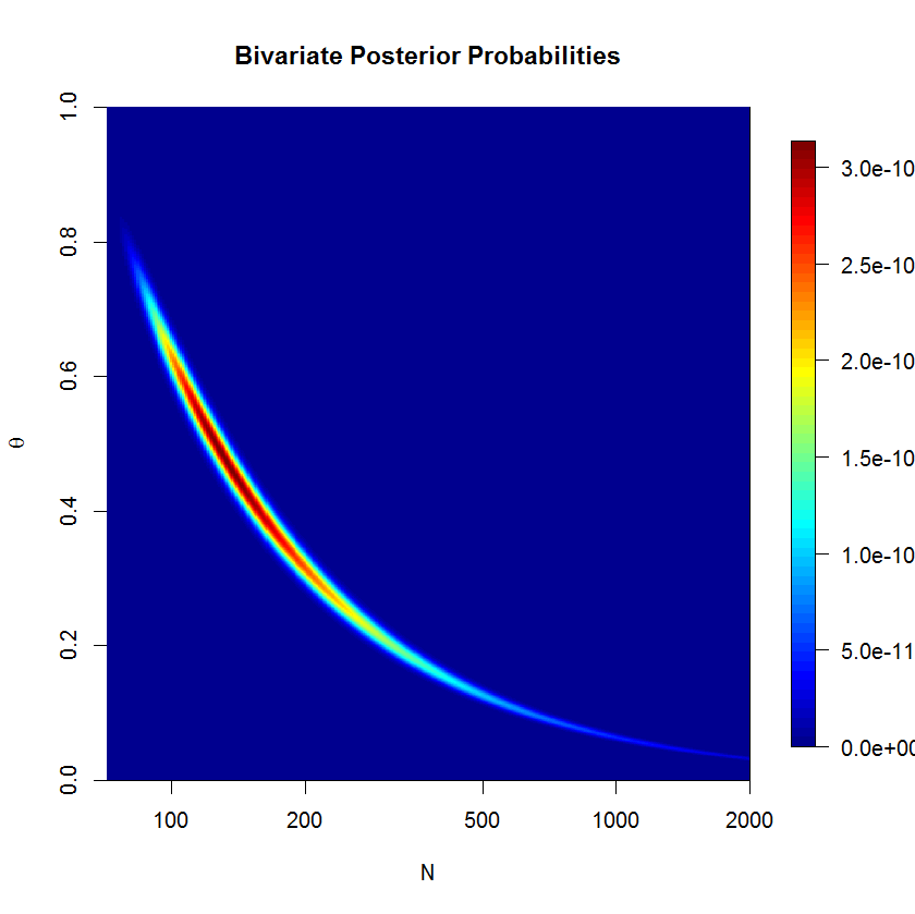
To check whether the rstan sampler is a problem or not, I computed the posterior over a grid. We can see that the posterior is banana-shaped; this kind of posterior can be problematic for euclidian metric HMC. But let's check the numerical results. (The severity of the banana shape is actually suppressed here since $N$ is on the log scale.) If you think about the banana shape for a minute, you'll realize that it must lie on the line $\bar{y}=\theta N$.

The code below may confirm that our results from stan make sense.

theta   <- seq(0+1e-10,1-1e-10, len=1e2)
N       <- round(seq(72, 5e5, len=1e5)); N[2]-N[1]
grid    <- expand.grid(N,theta)
y   <- c(53,57,66,67,72)
raftery.prob    <- function(x, z=y){
    N       <- x[1]
    theta   <- x[2]
    exp(sum(dbinom(z, size=N, prob=theta, log=T)))/N
}

post    <- matrix(apply(grid, 1, raftery.prob), nrow=length(N), 
                  ncol=length(theta), byrow=FALSE)    
approx(y=N, x=cumsum(rowSums(post))/sum(rowSums(post)), xout=0.975)
$x
[1] 0.975

$y
[1] 3236.665

Hm. This is not quite what I would have expected. Grid evaluation for the 97.5% quantile is closer to the JAGS results than to the rstan results. At the same time, I don't believe that the grid results should be taken as gospel because grid evaluation is making several rather coarse simplifications: grid resolution isn't too fine on the one hand, while on the other, we are (falsely) asserting that total probability in the grid must be 1, since we must draw a boundary (and finite grid points) for the problem to be computable (I'm still waiting on infinite RAM). In truth, our model has positive probability over $(0,1)\times\left\{N|N\in\mathbb{Z}\land N\ge72)\right\}$. But perhaps something more subtle is at play here.

Answer 2

Thanks again to @StéphaneLaurent and @user777 for their valuable input in the comments. After some tweaking of the prior for $\lambda$ I can now replicate the results from the paper of Raftery (1988).

Here is my analysis script and results using JAGS and R:

    # Load packages
    #===============================================================================================================
    
sapply(c("ggplot2"
         , "rjags"
         , "R2jags"
         , "hdrcde"
         , "runjags"
         , "mcmcplots"
         , "KernSmooth"), library, character.only = TRUE)

#===============================================================================================================
# Model file
#===============================================================================================================

cat("
    model {

    # Likelihood    
    for (i in 1:N) {
      x[i] ~ dbin(theta, n)
    }
    
    # Prior       
    n ~ dpois(mu)
    lambda ~ dgamma(0.005, 0.005)
#     lambda ~ dunif(0, 1000)
    mu <- lambda/theta
    theta ~ dunif(0, 1)    
}    
", file="jags_model_binomial.txt")


#===============================================================================================================
# Data
#===============================================================================================================

data.list <- list(x = c(53, 57, 66, 67, 72, NA), N = 6) # Waterbuck example from Raftery (1988)

#===============================================================================================================
# Inits
#===============================================================================================================

jags.inits <- function() { 
  list(
    n = sample(max(data.list$x, na.rm = TRUE):1000, size = 1) 
    , theta = runif(1, 0, 1)
    , lambda = runif(1, 1, 10)
#     , cauchy  = runif(1, 1, 1000)
    #     , mu = runif(1, 0, 5)
  )
}



#===============================================================================================================
    # Run the chains
    #===============================================================================================================
    
    # Parameters to store
    
params <- c("n"
            , "theta"
            , "lambda"
            , "mu"
            , paste("x[", which(is.na(data.list[["x"]])), "]", sep = "")
)

# MCMC settings

niter <- 500000 # number of iterations
nburn <- 20000  # number of iterations to discard (the burn-in-period)
nchains <- 5    # number of chains

# Run JAGS

out <- jags(
  data                 = data.list
  , parameters.to.save = params
  , model.file         = "jags_model_binomial.txt"
  , n.chains           = nchains
  , n.iter             = niter
  , n.burnin           = nburn
  , n.thin             = 50
  , inits              = jags.inits
  , progress.bar       = "text")

Computation took around 98 seconds on my desktop pc.

    # Inspect results
    #===============================================================================================================
    
print(out
      , digits = 2
      , intervals = c(0.025, 0.1, 0.25, 0.5, 0.75, 0.9,  0.975))

The results are:

Inference for Bugs model at "jags_model_binomial.txt", fit using jags,
 5 chains, each with 5e+05 iterations (first 20000 discarded), n.thin = 50
 n.sims = 48000 iterations saved
         mu.vect sd.vect  2.5%    10%    25%    50%    75%     90%   97.5% Rhat n.eff
lambda     62.90    5.18 53.09  56.47  59.45  62.74  66.19   69.49   73.49    1 48000
mu        521.28  968.41 92.31 113.02 148.00 232.87 467.10 1058.17 3014.82    1  1600
n         521.73  968.54 95.00 114.00 148.00 233.00 467.00 1060.10 3028.00    1  1600
theta       0.29    0.18  0.02   0.06   0.13   0.27   0.42    0.55    0.66    1  1600
x[6]       63.03    7.33 49.00  54.00  58.00  63.00  68.00   72.00   78.00    1 36000
deviance   34.88    1.53 33.63  33.70  33.85  34.34  35.34   36.81   39.07    1 48000

The posterior mean of $N$ is $522$ and the posterior median is $233$. I calculated the posterior mode of $N$ on the log-scale and back-transformed the estimate:

jagsfit.mcmc <- as.mcmc(out)
jagsfit.mcmc <- combine.mcmc(jagsfit.mcmc)

hpd.80 <- hdr.den(log(as.vector(jagsfit.mcmc[, "n"])), prob = c(80), den = bkde(log(as.vector(jagsfit.mcmc[, "n"])), gridsize = 10000))

exp(hpd.80$mode)

[1] 149.8161

And the 80%-HPD of $N$ is:

(hpd.ints <- HPDinterval(jagsfit.mcmc, prob = c(0.8)))

               lower      upper
deviance 33.61011007  35.677810
lambda   56.08842502  69.089507
mu       72.42307587 580.027182
n        78.00000000 578.000000
theta     0.01026193   0.465714
x[6]     53.00000000  71.000000

The posterior mode for $N$ is $150$ and the 80%-HPD is $(78; 578)$ which is very close to the limits given in the paper which are $(80; 598)$.