Interpretation of multiple logistic regression with interactions in R

Question

I am trying to look at whether 2 variables (one dichotomous categorical and one continuous) predict the occurrence of a dichotomous categorical dependent variable.

dependent variable is LENIpos - 0 = no event, 1 = event
predictor variables are Hip.Prox.Femur - 0 = no hip fracture, 1 = hip fracture
                and     age (continuous)

Both predictor variables have significant p values in separate chi square test and Mann Whitney U test respectively.

When I run a logistic regression glm(LENIpos ~ age + Hip.Prox.Femur, family = "binomial), the variables come out as not significant. (1)

However, when I run the logistic regression with interactions glm(LENIpos ~ age * Hip.Prox.Femur...) (2), they are no both significant. How is this to be interpreted?

Example R outputs:

(1)

Call: glm(formula = LENIpos ~ age + Hip.Prox.Fem, family = "binomial", 
    data = dvt)

Deviance Residuals: 
     Min       1Q   Median       3Q      Max  
 -0.9346  -0.7826  -0.4952  -0.3374   2.1897  

Coefficients:
                         Estimate Std. Error z value Pr(>|z|)   
(Intercept)              -3.46888    1.00693  -3.445 0.000571 ***
age                       0.02122    0.01519   1.397 0.162535  
Hip.Prox.Femhip fracture  0.72410    0.57790   1.253 0.210212    

(Dispersion parameter for binomial family taken to be 1)

    Null deviance: 145.23  on 151  degrees of freedom
Residual deviance: 135.48  on 149  degrees of freedom
AIC: 141.48

Number of Fisher Scoring iterations: 5

(2)

glm(formula = LENIpos ~ age * Hip.Prox.Fem, family = "binomial", 
    data = dvt)

Deviance Residuals: 
        Min       1Q   Median       3Q      Max  
    -1.0364  -0.7815  -0.5373  -0.1761   2.3443  

Coefficients:
                             Estimate Std. Error z value Pr(>|z|)  
(Intercept)                  -5.89984    1.98289  -2.975  0.00293 **
age                           0.05851    0.02818   2.076  0.03788 * 
Hip.Prox.Femhip fracture      5.04990    2.46269   2.051  0.04031 * 
age:Hip.Prox.Femhip fracture -0.06058    0.03339  -1.814  0.06965 . 


(Dispersion parameter for binomial family taken to be 1)

    Null deviance: 145.23  on 151  degrees of freedom
Residual deviance: 131.82  on 148  degrees of freedom
AIC: 139.82

Number of Fisher Scoring iterations: 6

Answer 1

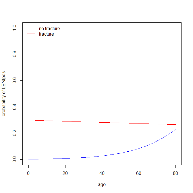
The relation of age or Hip.Prox.Femhip to the probability of LENIpos depends on the value of the other variable. That is suggested by the interaction term in your second model. In the usual R presentaton of regression coefficients, the coefficient for age in the second model is the relation of LENIpos to age in the absence of fracture, and the interaction term (age:Hip.Prox.Femhip fracture) is the difference from that relation in the presence of fracture. So the data seem consistent with age having a relation toLENIpos in the absence of fracture, but not in the presence of fracture. Plots of the +/- fracture subsets should help clarify this.

Answer 2

@EdM is right. The fact that the interaction's p-value is .06 (i.e., 'not-significant') is meaningless; you have an interaction. Let me add a few more details to supplement his (?) answer:

• A Mann-Whitney U-test of age~LENIpos isn't really the same as the univariate logistic regression of LENIpos~age (although the p-values will almost always be both significant or both not). You would do better to assess the univariate association by running the logistic regression.

• In R, a multiple linear regression comes with a global F-test of the model by default, but a multiple logistic regression does not (unfortunately). However, you can get a global test by assessing the difference between the null and residual deviances against a chi-squared distribution with the degrees of freedom equal to the difference between the null and residual dfs. Here is the test for your first model:

  > pchisq(q=145.23-135.48, df=151-149, lower.tail=FALSE)
  [1] 0.007635094
  

  So it is clear that your first model is significant.

• This seeming paradox (both univariate analyses significant, and the two predictor model significant even though neither predictor itself is significant) has a hidden cause: Your two predictors are themselves correlated. (The general name for this is multicollinearity.) As a result, the model doesn't know which of the two to attribute the association and expands both standard errors to acknowledge this fact.

  (Note that the preceding discussion ignores the existence of the interaction.)

---

• As @EdM states, plotting these functions can help you understand the interaction. Here is a basic plot with your output:

  lo.to.p = function(lo){
    odds = exp(lo)
    prob = odds / (odds+1)
    return(prob)
  }
  age   = 0:80
  lo.no =  -5.89984 + 0.05851*age
  lo.fr = (-5.89984 + 5.04990) + (0.05851 + -0.06058)*age
  p.no  = lo.to.p(lo.no)
  p.fr  = lo.to.p(lo.fr)
  
  windows()
    plot( age, p.no, col="blue", type="l", ylim=c(0,1), ylab="probability of LENIpos")
    lines(age, p.fr, col="red")
    legend("topleft", legend=c("no fracture", "fracture"), lty=1, col=c("blue","red"))