Geometric interpretation of multiple correlation coefficient $R$ and coefficient of determination $R^2$

Question

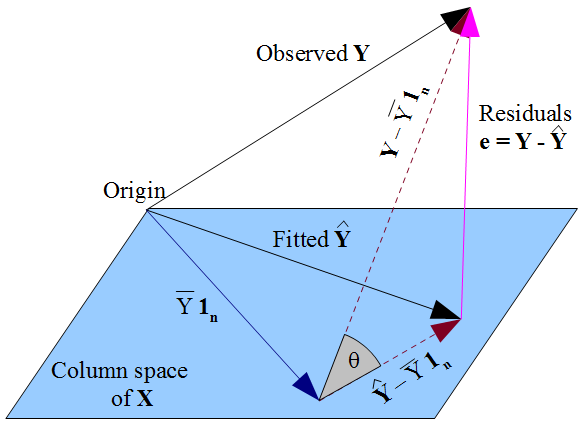
I am interested in the geometric meaning of the multiple correlation $R$ and coefficient of determination $R^2$ in the regression $y_i = \beta_1 + \beta_2 x_{2,i} + \dots + \beta_k x_{k,i} + \epsilon_i $, or in vector notation,

$$\mathbf{y} = \mathbf{X \beta} + \mathbf{\epsilon}$$

Here the design matrix $\mathbf{X}$ has $n$ rows and $k$ columns, of which the first is $\mathbf{x}_1 = \mathbf{1}_n$, a vector of 1s that corresponds to the intercept $\beta_1$.

The geometry is more interesting in the $n$-dimensional subject space rather than in the $k$-dimensional variable space. Define the hat matrix:

$$\mathbf{H} = \mathbf{X \left(X^\top X \right)}^{-1} \mathbf{X}^\top$$

This is an orthogonal projection onto the column space of $\mathbf{X}$, i.e. the flat through the origin spanned by the $k$ vectors representing each variable $\mathbf{x}_i$, the first of which is $\mathbf{1}_n$. Then $\mathbf{H}$ projects the vector of observed responses $\mathbf{y}$ onto its "shadow" on the flat, the vector of fitted values $\mathbf{\hat{y}} = \mathbf{Hy}$, and if we look along the path of the projection we see the vector of residuals $\mathbf{e} = \mathbf{y} - \mathbf{\hat{y}}$ forms the third side of a triangle. This should furnish us with two routes to a geometric interpretation of $R^2$:

1. The square of the multiple correlation coefficient, $R$, which is defined as the correlation between $\mathbf{y}$ and $\mathbf{\hat{y}}$. This will appear geometrically as the cosine of an angle.
2. In terms of lengths of vectors: for instance $SS_\text{residual} = \sum_{i=1}^{n}e_i^2 = \|\mathbf{e}\|^2$.

I would be delighted to see a brief account which explains:

• The finer details for (1) and (2),
• Why (1) and (2) are equivalent,
• Briefly, how the geometric insight lets us visualise basic properties of $R^2$, for instance why it goes to 1 when the noise variance goes to 0. (After all, if we can't intuit from our visualisation then it's no more than a pretty picture.)

I appreciate this is more straightforward if the variables are centred first, which removes the intercept from the question. However, in most textbook accounts which introduce multiple regression, the design matrix $\mathbf{X}$ is as I laid out. Of course it's fine if an exposition delves into the space spanned by the centred variables, but for insight into the textbook linear algebra, it would be very helpful to relate this back to what's happening geometrically in the uncentred situation. A really insightful answer might explain what exactly is breaking down geometrically when the intercept term is dropped - i.e. when the vector $\mathbf{1}_n$ is removed from the spanning set. I don't think this last point can be addressed by considering the centred variables alone.

Answer 1

If there is a constant term in the model then $\mathbf{1_n}$ lies in the column space of $\mathbf{X}$ (as does $\bar{Y}\mathbf{1_n}$, which will come in useful later). The fitted $\mathbf{\hat{Y}}$ is the orthogonal projection of the observed $\mathbf{Y}$ onto the flat formed by that column space. This means the vector of residuals $\mathbf{e} = \mathbf{y} - \mathbf{\hat{y}}$ is perpendicular to the flat, and hence to $\mathbf{1_n}$. Considering the dot product we can see $\sum_{i=1}^n e_i = 0$, so the components of $\mathbf{e}$ must sum to zero. Since $Y_i = \hat{Y_i} + e_i$ we conclude that $\sum_{i=1}^n Y_i = \sum_{i=1}^n \hat{Y_i}$ so that both fitted and observed responses have mean $\bar{Y}$.

The dashed lines in the diagram represent $\mathbf{Y} - \bar{Y}\mathbf{1_n}$ and $\mathbf{\hat{Y}} - \bar{Y}\mathbf{1_n}$, which are the centered vectors for the observed and fitted responses. The cosine of the angle $\theta$ between these vectors will therefore be the correlation of $Y$ and $\hat{Y}$, which by definition is the multiple correlation coefficient $R$. The triangle these vectors form with the vector of residuals is right-angled since $\mathbf{\hat{Y}} - \bar{Y}\mathbf{1_n}$ lies in the flat but $\mathbf{e}$ is orthogonal to it. Hence:

$$R = \cos(\theta) = \frac{\text{adj}}{\text{hyp}} = \frac{\|\mathbf{\hat{Y}} - \bar{Y}\mathbf{1_n}\|}{\|\mathbf{Y} - \bar{Y}\mathbf{1_n}\|} $$

We could also apply Pythagoras to the triangle:

$$\|\mathbf{Y} - \bar{Y}\mathbf{1_n}\|^2 = \|\mathbf{Y} - \mathbf{\hat{Y}}\|^2 + \|\mathbf{\hat{Y}} - \bar{Y}\mathbf{1_n}\|^2 $$

Which may be more familiar as:

$$\sum_{i=1}^{n} (Y_i - \bar{Y})^2 = \sum_{i=1}^{n} (Y_i - \hat{Y}_i)^2 + \sum_{i=1}^{n} (\hat{Y}_i - \bar{Y})^2 $$

This is the decomposition of the sums of squares, $SS_{\text{total}} = SS_{\text{residual}} + SS_{\text{regression}}$.

The standard definition for the coefficient of determination is:

$$R^2 = 1 - \frac{SS_{\text{residual}}}{SS_{\text{total}}} = 1 - \frac{\sum_{i=1}^n (y_i - \hat{y}_i)^2}{\sum_{i=1}^n (y_i - \bar{y})^2} = 1 - \frac{\|\mathbf{Y} - \mathbf{\hat{Y}}\|^2}{\|\mathbf{Y} - \bar{Y}\mathbf{1_n}\|^2}$$

When the sums of squares can be partitioned, it takes some straightforward algebra to show this is equivalent to the "proportion of variance explained" formulation,

$$R^2 = \frac{SS_{\text{regression}}}{SS_{\text{total}}} = \frac{\sum_{i=1}^n (\hat{y}_i - \bar{y})^2}{\sum_{i=1}^n (y_i - \bar{y})^2} = \frac{\|\mathbf{\hat{Y}} - \bar{Y}\mathbf{1_n}\|^2}{\|\mathbf{Y} - \bar{Y}\mathbf{1_n}\|^2}$$

There is a geometric way of seeing this from the triangle, with minimal algebra. The definitional formula gives $R^2 = 1 - \sin^2(\theta)$ and with basic trigonometry we can simplify this to $\cos^2(\theta)$. This is the link between $R^2$ and $R$.

Note how vital it was for this analysis to have fitted an intercept term, so that $\mathbf{1_n}$ was in the column space. Without this, the residuals would not have summed to zero, and the mean of the fitted values would not have coincided with the mean of $Y$. In that case we couldn't have drawn the triangle; the sums of squares would not have decomposed in a Pythagorean manner; $R^2$ would not have had the frequently-quoted form $SS_{\text{reg}}/SS_{\text{total}}$ nor be the square of $R$. In this situation, some software (including R) uses a different formula for $R^2$ altogether.