5
$\begingroup$

Suppose I wish to fit $\hat{y} = \beta_0 + \beta_1x$ where the the data is as follows:

x = 0.0, 0.1, 0.2, 0.3, 0.4
y = 0.0, 0.0, 0.0, 0.0, 0.0

Clearly, $\hat{\beta_1} = 0$ and $\hat{\beta_0} = 0$. But what is $R^2$ in this instance?

Suppose I calculate:

$$r = \frac{n S_{xy} - S_xS_y}{\sqrt{(nS_{xx} - S_x^2) (nS_{yy} - S_y^2)}}$$

or,

$$R^2 = 1 - \frac{SS_{res}}{SS_{tot}}$$

Then both will be NaN/Undefined since the denominator in both instances will be zero.

So, for this particular dataset, is $R^2$ actually defined? I would hesitate to guess that it should be 1, given the data fits the model perfectly?

$\endgroup$
0

3 Answers 3

9
$\begingroup$

The following plots are accompanied by their Pearson product-moment correlation coefficients (image credit):
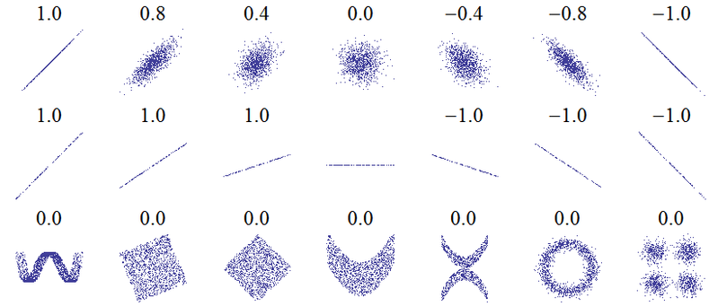
Pearson correlation for various scatter plots

If the points lie exactly on an upwards sloping line then the Pearson correlation is +1, if they lie exactly on a downwards sloping line the correlation is -1. But notice that the horizontal line has an undefined correlation.

At first sight you might expect this to be zero, as a compromise between +1 and -1. You may have thought that since positive correlation means "as one variable increases, the other tends to increase" while negative correlation means "as one variable increases, the others tends to decrease", the fact that $Y$ neither tends to increase nor decrease as $X$ increases means that $r=0$. That idea is correct for the other plots labelled $r=0$, but they all exhibited variation in $Y$. Correlation is symmetric: the correlation between $X$ and $Y$ is the same as that between $Y$ and $X$. Turning things around, in the $r=0$ plots we see that as $Y$ increases, $X$ neither tends to increase nor decrease. But in our case what happens to $X$ as $Y$ changes? We just don't know! We certainly can't claim (as $r=0$ would imply) that $X$ would neither tend to increase nor decrease. We never got a chance to see it, because $Y$ never varied. Intuitively, there's no way we can determine the correlation from the available data.

More technically, consideration of the formula for PMCC should clarify things:

$$r = \frac{\text{Covariance of X and Y}}{\text{SD of X} \times \text{SD of Y}}$$

where "SD" stands for standard deviation. On a completely horizontal line, the standard deviation of $Y$ is zero because that variable does not vary at all. So we have zero on the denominator. Also since $X$ and $Y$ can not co-vary, then the covariance is zero, and the numerator is zero also. Hence the fraction is $\frac{0}{0}$ which is an indeterminate form and so the correlation coefficient is not defined.

In a simple linear regression model (only one response and one predictor variable plus an intercept), the coefficient of determination $R^2$ is simply the square of $r$, the PMCC between $X$ and $Y$. Unsurprisingly, this will not be defined either. This is intuitive if we think about $R^2$ as the proportion of variance explained - here the response variable has no variation, so we can explain 0 out of 0 variance, which as a proportion brings us back to the indeterminate form $\frac{0}{0}$.

This conclusion holds true regardless of whether the recorded data are all identically zero, or identically some other number, so long as it would give a horizontal line in a graph of $Y$ against $X$. Note that there may be a difference between the "true" values of $Y$ and those that have been recorded in the data set to the specified level of accuracy. It's possible in a case such as yours that the correct values of $Y$ all round to 0.0 to one decimal place, but if we had access to them to full accuracy, we may be able to observe very small deviations about 0. If that were the case then the actual PMCC and coefficient of determination would both exist, and (i) be approximately equal to zero if the small deviations were just "noise", (ii) be anything up to and including 1 if the small deviations formed an increasing trend indiscernible at the current level of accuracy, or (iii) be anything up to and including $r = -1$ and $R^2 = 1$ if they formed a currently indiscernible downwards trend.

In this answer I have only considered the case of simple linear regression, where the response depends on one explanatory variable. But the argument also applies to multiple regression, where there are several explanatory variables. I'll assume the model includes an intercept term, since dropping the intercept is rarely a good idea and even with a model without an intercept, it's unlikely you want to calculate $R^2$. So long as the intercept is included in the model, then $R^2$ is just the square of multiple correlation coefficient $R$, which is the PMCC between the observed values of the response $Y$ and the values fitted by the model. If $Y$ shows no variation (at least to the recorded accuracy) then the same considerations prevent you calculating $R$ and hence $R^2$.

$\endgroup$
2
$\begingroup$

As $R^2$ is "variance explained", then as $0 = 0 + 0 \times x$ has variance of 0, the same as variance of $y$, so we could think of it as 100% variance explained, i.e. $R^2 = 1$. On another hand, as you notice $0/0$ is indeterminate and does not make sense, as this model does not either. As goangit mentioned, this kind of model doesn't meet criteria for regression and it is not even a linear function of $x$, but rather a constant function, so by definition this is not a regression problem.

$\endgroup$
2
  • 3
    $\begingroup$ $0$ is a linear function. However, this is irrelevant, because what matters is whether $y$ is a linear function of the parameters--which it also is. This model is a perfectly fine regression model and the data are perfectly fine for applying a regression model. $\endgroup$
    – whuber
    Commented Dec 3, 2014 at 21:54
  • 3
    $\begingroup$ I'd submit that "we get 100% variance explained" isn't true. Thinking about $R^2$ as "percentage variance explained", we have explained 0 out of a total of 0 variance. The fraction of variance explained is $\frac{0}{0}$ - this is an indeterminate form so does not correspond to 100%. The model itself does make sense, but the attempt to calculate $R^2$ does not. $\endgroup$
    – Silverfish
    Commented Dec 3, 2014 at 22:20
0
$\begingroup$

For the General Linear Model to be suitable the data need to meet certain criteria:

  1. The mean response is a linear function of the predictors.
  2. Model residuals are conditionally independent.
  3. Model residuals are distributed with conditional mean zero.
  4. Model residuals have constant conditional variance.
  5. Model residuals are conditionally normal in distribution.

The response you describe fails to meet (at least) criterion 5, so the General Linear Model does not apply to this example.

As discussed in the comments, this does not prevent the calculation of RSS, which you have already noted is 0/0, an indeterminate form.

$\endgroup$
6
  • 4
    $\begingroup$ I don't agree with 5 being a prerequisite for regression analysis. Gauss–Markov theorem still applies even if residuals aren't normal, for instance, though lack of normality can have other impacts on interpretation of results (t tests, confidence intervals etc). $\endgroup$
    – Silverfish
    Commented Dec 3, 2014 at 9:42
  • 4
    $\begingroup$ Incidentally, it's possible there is Gaussian (normally distributed) noise - the data is recorded to an accuracy of one decimal place, so a Gaussian disturbance of order $10^{-3}$ wouldn't show up in the data. This is an extreme example of the fact that data recorded to a finite accuracy can't have strictly normal errors. $\endgroup$
    – Silverfish
    Commented Dec 3, 2014 at 10:00
  • 2
    $\begingroup$ I agree with @Silverfish. #5 is a complete red herring here. If I had data generated by $y = a + bx +$ uniform noise, and want to get $a$ and $b$ would you say that it's not a regression problem because the noise is uniform not normal? How would you tackle it then? In fact, I don't think #5 ever applies to real data! $\endgroup$
    – Nick Cox
    Commented Dec 3, 2014 at 11:55
  • $\begingroup$ Interesting. Sure, regression can be performed with all kinds of residual distributions, and #5 is not related to the calculation of RSS. The problem is degenerate and R^2 = 0/0 is indeterminate and #5 is not the correct criterion for rejecting the calculation of RSS. As @Silverfish says, #5 relates to the evaluation and interpretation of estimated quantities like p-values and confidence limits, quantities that render the General Linear Model useful for inference and not merely regression. $\endgroup$
    – goangit
    Commented Dec 3, 2014 at 13:25
  • 3
    $\begingroup$ The exact form of the conditional distribution remains irrelevant to explaining how to think about $r^2$ here. It isn't needed in any explanation, as shown by the other answers. $\endgroup$
    – Nick Cox
    Commented Dec 3, 2014 at 20:00

Your Answer

By clicking “Post Your Answer”, you agree to our terms of service and acknowledge you have read our privacy policy.

Not the answer you're looking for? Browse other questions tagged or ask your own question.